Chapter 4 An Illustrative Example of Case 2 Best–Worst Scaling
Authors: Hideo Aizaki and James Fogarty
Latest Revision: 29 August 2019 (First Release: 30 March 2018)
4.1 Before you get started
This tutorial, which is a revised version of the manual for the package support.BWS2, presents the entire process of Case 2 (profile case) best–worst scaling (BWS)—from constructing the profiles to analyzing responses using R (R Core Team 2021b). The tutorial assumes some familiarity with R. If you are completely unfamiliar with R, you are advised to consult R Core Team (2021a) and the other support materials before attempting the material below.
NOTE: this tutorial is based on the support.BWS2 package version 0.2-2 or later.
4.2 Overview of Case 2 BWS
This section explain Case 2 BWS briefly. For complete details on the approach please refer to works such as Flynn et al. (2007), Flynn et al. (2008), Louviere, Flynn, and Marley (2015), and Marley, Flynn, and Louviere (2008). For an outline of three variants of BWS, see Section 3.2.
Each Case 2 BWS question has a profile that has three or more attributes and each attribute has two or more levels. The profile is expressed as a combination of attribute-levels. Numerous profiles are constructed using experimental designs. Each profile’s attributes are fixed, but the combination of attribute-levels in each profile changes according to the profile. A profile selected from all the constructed profiles is presented to respondents, who are then asked to choose the best and worst attribute-levels. This style of question is repeated until all the profiles are evaluated.
One basic approach for constructing profiles is the orthogonal main-effect design (OMED). The OMED approach can be understood as follows. Assume that the profiles have \(K\) attributes and each attribute has \(L_{k}\) levels. If all the attributes have the same number of levels, \(L\), a \(L^{K}\) OMED is used to construct the profiles. In this case the columns of the OMED correspond to attributes, while the rows correspond to profiles.
By analyzing the responses to Case 2 BWS questions it is possible to measure the preferences of respondents for the different attribute-levels. There are two approaches for analyzing the responses: the counting approach and the modeling approach.
The counting approach calculates scores based on the number of times (frequency or count) attribute-level \(i\) is selected as the best (\(B_{in}\): B score for attribute-level \(i\)) and the worst (\(W_{in}\): W score for attribute-level \(i\)) among all the questions for respondent \(n\). A (disaggregated) best-minus-worst (BW) score and its standardized variant are defined as: \[\begin{equation} BW_{in} = B_{in} - W_{in}, \label{eq:disagbwscore} \end{equation}\] and \[\begin{equation} std. BW_{in} = \frac{BW_{in}}{f_{i}}, \label{eq:stddisagbwscore} \end{equation}\] where \(f_{i}\) is the frequency with which attribute-level \(i\) appears across all questions. These scores reveal respondents’ preferences for attribute-levels.
The modeling approach uses discrete choice models to analyze the responses. When using the modeling approach, a model type must be selected according to the assumptions made about the respondents’ choices to the Case 2 BWS questions. Then, the dataset must be formatted as per the selected model. There are three standard models of analysis: paired, marginal, and marginal sequential models (Flynn et al. 2007, 2008; Hensher, Rose, and Greene 2015; Louviere, Flynn, and Marley 2015). Although the three models all assume that respondents derive utility from each attribute-level in a profile, the assumption regarding how they select the best and worst attribute-levels from the set of attribute-levels shown in the profile differs across the three models.
The paired model assumes that respondents select an attribute-level as the best and another attribute-level as the worst because the difference in utility between the two attribute-levels represents the greatest utility difference among all the utility differences. The number of utility differences in a pair is equal to the number of possible pairs in which attribute-level \(i\) is selected as the best and attribute-level \(j\) is selected as the worst (\(i \neq j\)) from \(K\) attribute-levels, that is, \(K \times (K - 1)\).
The marginal model assumes that there are \(K\) possible best attribute-levels and \(K\) possible worst attribute-levels in a profile. That means that attribute-level \(i\) is selected as the best from \(K\) possible best attribute-levels in the profile, and that attribute-level \(j\) is selected as the worst from \(K\) possible worst attribute-levels. This is because the model considers that the utility for attribute-level \(i\) is the maximum among the utilities for \(K\) attribute-levels, and that the utility for attribute-level \(j\) is the minimum.
The marginal sequential model assumes that respondents select attribute-level \(i\) as the best from \(K\) attribute-levels in the profile, and that attribute-level \(j\) is selected as the worst from the remaining \(K - 1\) attribute-levels.
The probability of selecting attribute-level \(i\) as the best and attribute-level \(j\) (\(i \neq j\)) as the worst from a choice set \(C\) for each model can be expressed using the conditional logit model with the systematic component of utility \(v\), as follows.
- The paired model
\[\begin{equation} \mathrm{Pr}(\mathrm{best} = i, \mathrm{worst} = j) = \frac{\exp{(v_{i} - v_{j})}}{\sum_{p, q \subset C, p \neq q} \exp{(v_{p} - v_{q})}}. \end{equation}\]
- The marginal model
\[\begin{equation} \mathrm{Pr}(\mathrm{best} = i, \mathrm{worst} = j) = \frac{\exp{(v_{i})}}{\sum_{p \subset C} \exp{(v_{p})}}\frac{\exp{(-v_{j})}}{\sum_{p \subset C} \exp{(-v_{p})}}. \end{equation}\]
- The marginal sequential model
\[\begin{equation} \mathrm{Pr}(\mathrm{best} = i, \mathrm{worst} = j) = \frac{\exp{(v_{i})}}{\sum_{p \subset C} \exp{(v_{p})}}\frac{\exp{(-v_{j})}}{\sum_{q \subset C - i} \exp{(-v_{q})}}. \end{equation}\]
Each of three standard models is divided into subvariants (e.g., Al-Janabi, Flynn, and Coast 2011; Flynn et al. 2007; Hensher, Rose, and Greene 2015) according to the type of the independent variables included in the model (i.e., attribute variables and/or attribute level variables).
4.3 Packages for Case 2 BWS
We use three CRAN packages support.BWS2 (Aizaki 2019a; Aizaki and Fogarty 2019), DoE.base (Grömping 2018), and survival (Therneau 2020) to explain how to implement Case 2 BWS in R. The package support.BWS2 provides functions to convert an OMED into Case 2 BWS questions, create a dataset for the analysis from the OMED and the responses to the questions, and calculate BWS scores. The function oa.design() in the package DoE.base can construct OMEDs, whereas the function clogit() in the package survival can fit the conditional logit model, a basic discrete choice model. Instead of clogit(), mlogit() in the package mlogit (Croissant 2020b) or gmnl() in the package gmnl (Sarrias and Daziano 2017) can also be used for the conditional logit model analysis. Refer to the appendix 4A for code to convert a dataset prepared for clogit() into the format required for mlogit(). The latter two functions are also appropriate for advanced discrete choice models such as a mixed (random parameters) logit model. Details for the R packages regarding experimental designs (Groemping 2020) and discrete choice models (Zeileis 2020) can be found on CRAN.
Given the packages have been downloaded and installed, we then load the packages needed for the example into the current session:
Note that we printed out four digits in the example. To set the same appearance format in R, you need to execute the following code line in your current session.
4.4 Designing a choice situation
We explains how to use the functions on the basis of a survey regarding potential tourists’ valuation of agritourism. Agritourism refers to various activities offered by farms to visitors, such as hands-on farm work or outdoor recreation. In the survey, a total of 240 respondents were asked to evaluate agritourism packages provided by dairy farms (ranches) in Hokkaido, Japan. As the first step of implementing Case 2 BWS, it is necessary to determine the features of agritourism that are potentially available. In this example the agritourism package consists of the following four types of activities, each with three activity items (variable names are in parenthesis):
- Hands-on ranch chores (
chore)- Milking a cow (
milking) - Feeding a cow (
feeding) - Nursing a calf (
nursing)
- Milking a cow (
- Hands-on food processing (
food)- Butter making (
butter) - Ice-cream making (
ice) - Creamy caramel making (
caramel)
- Butter making (
- Hands-on craft making (
craft)- Making a product from wool (
wool) - Making a product from wood (
wood) - Making a product from pressed flowers (
flower)
- Making a product from wool (
- Outdoor activities (
outdoor)- Horse riding (
horse) - Tractor riding (
tractor) - Walking with cows (
cow)
- Horse riding (
Each BWS question asked respondents to select the most and least interesting of the four activities shown in the question.
4.5 Generating an OMED
The second step is to prepare an OMED corresponding to the choice situation. For the survey, we created a \(3^{4}\) OMED using the function oa.design(). Although the function has many arguments, we used nlevels and randomize in this example. The simple call to the function is:
with its arguments:
nlevels: A vector containing the number of levels corresponding to the OMED that you wish to create.randomize: A logical variable denoted byTRUEwhen randomizing the order of the rows in the resultant design orFALSEwhen not doing so.
The following lines of code create the \(3^{4}\) OMED used in the survey and store it in the object des:
##   A B C D
## 1 1 1 1 1
## 2 1 2 3 2
## 3 1 3 2 3
## 4 2 1 3 3
## 5 2 2 2 1
## 6 2 3 1 2
## 7 3 1 2 2
## 8 3 2 1 3
## 9 3 3 3 1
The resultant design has nine rows, meaning that there are nine BWS questions. Note that randomize was set to FALSE so that the OMED was reproducible. However, the survey randomized the order of rows in the design. Note that the above code converts the resultant OMED into a matrix with elements expressed by integer values using the function data.matrix(). This step is needed because the function oa.design() returns the design in data frame format, in which each variable (column) is stored in factor format. The factor format is not compatible with the functions in the support.BWS2 package.
4.6 Creating questions
The third step is to create Case 2 BWS questions. The bws2.questionnaire() function converts an OMED into a series of Case 2 BWS questions, and then displays the resultant questions on an R console. A generic call to the function is:
with its arguments:
choice.sets: A data frame or matrix containing an OMED.attribute.levels: A list containing the names of attributes and their levels.position: A character showing the position where attribute-levels are shown in questions.
In preparation for analysis, the names of the attributes (activities) and attribute-levels (activity items) are stored in the list attr.lev:
attr.lev <- list(
   chore = c("milking", "feeding", "nursing"),
   food = c("butter", "ice", "caramel"),
   craft = c("wool", "wood", "flower"),
   outdoor = c("horse", "tractor", "cow"))
Then, we convert the data into a series of Case 2 BWS questions from the OMED using the bws2.questionnaire() function:
bws2.questionnaire(choice.sets = des, attribute.levels = attr.lev,
   position = "left")

Q1
 Attribute Best Worst
 milking   [ ]  [ ]
 butter    [ ]  [ ]
 wool      [ ]  [ ]
 horse     [ ]  [ ]

 ...

Q9
 Attribute Best Worst
 nursing   [ ]  [ ]
 caramel   [ ]  [ ]
 flower    [ ]  [ ]
 horse     [ ]  [ ]
We can the copy the resultant questions from the R console, and then paste them into other software packages such as a word processor to create the actual questionnaire.
4.7 Conducting a survey
In practice the next step is to conduct the actual questionnaire survey using the Case 2 BWS questions created above. In this case, because the survey has already been conducted, this step is skipped here.
4.8 Creating a dataset
4.8.1 Preparing a dataset including responses to the questions
We need to create a dataset for the analysis by combining the OMED generated in the second step and the actual responses to the Case 2 BWS questions. The actual survey responses are stored in the dataset agritourism which is part of the support.BWS2 package. As such, the dataset is loaded into the current session as follows:
## [1] 240 21## [1] "id" "b1" "w1" "b2" "w2" "b3" "w3" "b4"
## [9] "w4" "b5" "w5" "b6" "w6" "b7" "w7" "b8"
## [17] "w8" "b9" "w9" "gender" "age"As shown above, the dataset contains 240 observations with 21 variables. The id variable is the respondents’ unique id variable. Response variables b1–w9 correspond to the Case 2 BWS questions: b denotes a response as the best, w denotes a response as the worst, and the numbers 1 to 9 indicate the BWS question number. The gender is the respondents’ gender variable: 1 denotes male, 2 denotes female. The age is the respondents’ age category variable, where: 2, 3, 4, and 5 correspond to age brackets of: 20s, 30s, 40s, and 50s, respectively.
When you conduct a survey, you would have to create a respondent dataset on the basis of the completed questionnaire. The structure of your respondent dataset needs to follow the basic structure of the agritourism dataset mentioned above: it must include the respondent’s identification number (id) variable in the first column; and the response variables must be in the subsequent columns, each indicating which attribute-levels are selected as the best and worst for each question. The response variables must be constructed such that the best attribute-levels alternate with the worst by question. For example, when there are nine BWS questions, the variables are \(b1\) \(w1\) \(b2\) \(w2\) … \(b9\) \(w9\). Here, \(b_{i}\) and \(w_{i}\) are the attribute-levels selected as the best and worst for the \(i\)-th question. The row numbers of the attribute-levels selected as the best and worst are stored in the response variables. For example, suppose a respondent was asked to answer Q1 mentioned above, and that the respondent selected milking (attribute-level in the first row) as the best and wool (attribute-level in the third row) as the worst. The response variables b1 and w1, corresponding to the respondent’s answer to this question, take values of 1 (= the attribute-level in the first row) and 3 (= the attribute-level in the third row). Other variables in the respondent dataset are treated as the respondents’ characteristics such as gender and age. The names of the id and response variables are left to the discretion of the user.
4.8.2 Combining the design and the responses
After finishing the preparation of the respondent dataset, a dataset for the analysis is created using the bws2.dataset() function (Step 6). The generic call to the function is:
bws2.dataset(data, id, responses, choice.sets, attribute.levels,
  base.attribute = NULL, base.level = NULL, reverse = TRUE, model = "paired")
with its arguments:
data: A data frame containing a respondent dataset.id: A character showing the name of the respondent’s identification number variable used in the respondent dataset.responses: A vector containing the names of response variables in the respondent dataset, showing the best and worst attribute-levels selected for each Case 2 BWS question.choice.sets: A data frame or matrix containing an OMED.attribute.levels: A list containing the names of the attributes and their levels.base.attribute: A character showing the base attribute: the argument is used when attribute variables are created as effect-coded ones andNULLis assigned to the argument when attribute variables are created as dummy-coded ones.base.level: A list containing the base level in each attribute: the argument is used when attribute level variables are created as effect-coded ones andNULLis assigned to the argument when attribute level variables are created as dummy-coded ones.reverse: A logical value denoted byTRUEwhen the signs of the attribute variables are reversed for the possible worst, or otherwiseFALSE.model: A character showing a type of dataset created by this function:"paired"for a paired model,"marginal"for a marginal model, and"sequential"for a marginal sequential model.
Note that the order of questions in the respondent dataset has to be the same as that in the OMED assigned to choice.sets.
In this example, we store the names of the response variables used in the respondent dataset agritourism in the vector response.vars. Note as we do not want the details from the first column we use:
##  [1] "b1" "w1" "b2" "w2" "b3" "w3" "b4" "w4" "b5" "w5" "b6" "w6" "b7" "w7" "b8"
## [16] "w8" "b9" "w9"
Furthermore, the base level in each attribute (assumed to be nursing for attribute chore, caramel for attribute food, flower for attribute craft, and cow for attribute outdoor) is stored in the object base.lev in list format:
base.lev <- list(
   chore = c("nursing"),
   food = c("caramel"),
   craft = c("flower"),
   outdoor = c("cow"))
The datasets for the paired, marginal, and marginal sequential models with both attribute and attribute-level variables (e.g., Flynn et al. 2007, 2008; Louviere, Flynn, and Marley 2015) are created using the function bws2.dataset(). The base.attribute, base.level, reverse, and model arguments are set according to the model variant we will use. The following lines of code create the datasets for these model variants:
# Dataset for the paired model
pr.data1 <- bws2.dataset(
   data = agritourism,
   id = "id",
   response = response.vars,
   choice.sets = des,
   attribute.levels = attr.lev,
   reverse = TRUE, # attribute variables = 1 for a possible best,
                   # -1 for a possible worst, and 0 otherwise
   base.level = base.lev, # effect-coded attribute-level variables
   model = "paired") # the paired model
# Dataset for the marginal model
mr.data1 <- bws2.dataset(
   data = agritourism,
   id = "id",
   response = response.vars,
   choice.sets = des,
   attribute.levels = attr.lev,
   reverse = TRUE,
   base.level = base.lev,
   model = "marginal") # the marginal model
# Dataset for the marginal sequential model
sq.data1 <- bws2.dataset(
   data = agritourism,
   id = "id",
   response = response.vars,
   choice.sets = des,
   attribute.levels = attr.lev,
   reverse = TRUE,
   base.level = base.lev,
   model = "sequential") # the marginal sequential model
The structure of the resultant dataset differs according to the model variants. The pr.data1 consists of 25,920 rows (= 240 respondents \(\times\) 9 questions \(\times\) 12 possible pairs per question) and 27 columns (variables):
## [1] 25920 27In this example, each question contains four attribute-levels, and thus the number of possible pairs per question is \(12\) (\(= 4 \times 3\)). The 27 variables are as follows:
##  [1] "id"       "Q"        "PAIR"     "BEST"     "WORST"    "BEST.AT"
##  [7] "WORST.AT" "BEST.LV"  "WORST.LV" "chore"    "food"     "craft"
## [13] "outdoor"  "milking"  "feeding"  "butter"   "ice"      "wool"
## [19] "wood"     "horse"    "tractor"  "RES.B"    "RES.W"    "RES"
## [25] "STR"      "gender"   "age"
The following displays the variables id, Q, BEST.LV, WORST.LV, and four attribute variables in the pr.data1 corresponding to the 12 possible pairs in the first question (Q = 1) for respondent 1 (id = 1). The variables BEST.LV and WORST.LV show the best and worst attribute-levels in a possible pair: the first row in the following indicates a possible pair in which milking, an attribute-level in hands-on ranch chores, is treated as the best and butter, an attribute-level in hands-on food processing, is treated as the worst. The attribute variables are created as attribute-specific constants with reversed sign when the attributes are treated as the possible worst (see the argument setting in code mentioned above: reverse = TRUE). Therefore, the first row indicates that the value of the attribute variable chore and that of food are 1 and -1, respectively, and the value of the remaining attribute variables such as craft and outdoor are 0.
##    id Q BEST.LV WORST.LV chore food craft outdoor
## 1   1 1 milking   butter     1   -1     0       0
## 2   1 1 milking     wool     1    0    -1       0
## 3   1 1 milking    horse     1    0     0      -1
## 4   1 1  butter  milking    -1    1     0       0
## 5   1 1  butter     wool     0    1    -1       0
## 6   1 1  butter    horse     0    1     0      -1
## 7   1 1    wool  milking    -1    0     1       0
## 8   1 1    wool   butter     0   -1     1       0
## 9   1 1    wool    horse     0    0     1      -1
## 10  1 1   horse  milking    -1    0     0       1
## 11  1 1   horse   butter     0   -1     0       1
## 12  1 1   horse     wool     0    0    -1       1
The following shows the eight attribute-level variables (from milking to tractor) and RES in the pr.data1 corresponding to the 12 rows mentioned above. The attribute-level variables are created as effect-coded variables (the base level in each attribute is assigned to the argument base.level in the code mentioned above). The signs for the effect-coded attribute-level variables are also reversed when attribute-levels are treated as the possible worst.
In this example, the first row indicates that the value of attribute-level variable milking and that of butter are 1 and -1, respectively, and the values of the remaining attribute-level variables are 0. The variable RES is a response variable, taking a value of 1 if a possible pair is actually selected by respondents from all the possible pairs, and 0 otherwise. In this example, the value of RES is 1 in the fifth row, and 0 in the remaining 11 rows. This means that respondent 1 selected a pair in which butter making is the best and making a product from wool is the worst.
##    id Q milking feeding butter ice wool wood horse tractor RES
## 1   1 1       1       0     -1   0    0    0     0       0   0
## 2   1 1       1       0      0   0   -1    0     0       0   0
## 3   1 1       1       0      0   0    0    0    -1       0   0
## 4   1 1      -1       0      1   0    0    0     0       0   0
## 5   1 1       0       0      1   0   -1    0     0       0   1
## 6   1 1       0       0      1   0    0    0    -1       0   0
## 7   1 1      -1       0      0   0    1    0     0       0   0
## 8   1 1       0       0     -1   0    1    0     0       0   0
## 9   1 1       0       0      0   0    1    0    -1       0   0
## 10  1 1      -1       0      0   0    0    0     1       0   0
## 11  1 1       0       0     -1   0    0    0     1       0   0
## 12  1 1       0       0      0   0   -1    0     1       0   0
The mr.data1 consists of 17,280 rows (= 240 respondents \(\times\) 9 questions \(\times\) 8 possible best and worst attribute-levels per question) and 26 columns:
## [1] 17280 26Each question contains four attribute-levels, and thus the number of the possible best and worst options per question in the marginal model is \(8\) (\(= 4\) possible best \(+\ 4\) possible worst). The 26 variables are as follows:
##  [1] "id"      "Q"       "ALT"     "BW"      "ATT.cha" "ATT"     "LEV.cha"
##  [8] "LEV"     "chore"   "food"    "craft"   "outdoor" "milking" "feeding"
## [15] "butter"  "ice"     "wool"    "wood"    "horse"   "tractor" "RES.B"
## [22] "RES.W"   "RES"     "STR"     "gender"  "age"
The following displays the variables id, Q, ALT, BW, LEV.cha, and four attribute variables in the mr.data1 corresponding to the eight possible best and worst options in the first question for respondent 1. The first four rows show the possible best (BW = 1), while the last four rows show the possible worst (BW = -1).
The variable LEV.cha shows the possible best and worst attribute-levels: the first row in the following indicates that milking, an attribute-level in hands-on ranch chores, is treated as the best option, while the last row indicates that horse, an attribute-level in outdoor, is treated as the worst option. The attribute variables are created as attribute-specific constants with reversed sign when the attributes are treated as the worst option. Therefore, the first row indicates that the value of the attribute variable chore is 1 and the values of the remaining attribute variables are 0; while the last row indicates that the value of the attribute variable outdoor is -1 and the values of the remaining attribute variables are 0.
##   id Q ALT BW LEV.cha chore food craft outdoor
## 1  1 1   1  1 milking     1    0     0       0
## 2  1 1   2  1  butter     0    1     0       0
## 3  1 1   3  1    wool     0    0     1       0
## 4  1 1   4  1   horse     0    0     0       1
## 5  1 1   1 -1 milking    -1    0     0       0
## 6  1 1   2 -1  butter     0   -1     0       0
## 7  1 1   3 -1    wool     0    0    -1       0
## 8  1 1   4 -1   horse     0    0     0      -1
The following displays the eight attribute-level variables and the variable RES in the mr.data1 corresponding to the eight rows mentioned above. The definition of the attribute-level variables in the mr.data1 is the same as that in the pr.data1: the first row shows that the value of milking is 1 and the value of the remaining attribute-level variables are 0, while the last row shows that the value of horse is -1 and the values of the remaining attribute-level variables are 0. According to the values of the RES, respondent 1 selected butter making as the best option and making a product from wool as the worst option in the first question.
##   LEV.cha milking feeding butter ice wool wood horse tractor RES
## 1 milking       1       0      0   0    0    0     0       0   0
## 2  butter       0       0      1   0    0    0     0       0   1
## 3    wool       0       0      0   0    1    0     0       0   0
## 4   horse       0       0      0   0    0    0     1       0   0
## 5 milking      -1       0      0   0    0    0     0       0   0
## 6  butter       0       0     -1   0    0    0     0       0   0
## 7    wool       0       0      0   0   -1    0     0       0   1
## 8   horse       0       0      0   0    0    0    -1       0   0
The sq.data1 consists of 15,120 rows (= 240 respondents \(\times\) 9 questions \(\times\) 7 possible best and worst attribute-levels per question) and 26 columns:
## [1] 15120 26Each question contains four attribute-levels, and thus the number of the possible best and worst options per question in the marginal sequential model is \(7\) (\(= 4\) possible best \(+\ 3\) possible worst). The 26 variables are the same as those in mr.data1:
##  [1] "id"      "Q"       "ALT"     "BW"      "ATT.cha" "ATT"     "LEV.cha"
##  [8] "LEV"     "chore"   "food"    "craft"   "outdoor" "milking" "feeding"
## [15] "butter"  "ice"     "wool"    "wood"    "horse"   "tractor" "RES.B"
## [22] "RES.W"   "RES"     "STR"     "gender"  "age"
The following shows a dataset corresponding to the first question for respondent 1. The row structure in sq.data1 is different from that in mr.data1: the first four rows correspond to the four possible best attribute levels in the first question (BW = 1), whereas the last three rows correspond to the three possible worst (BW = -1); the row corresponding to the attribute-level selected as the best by respondents is deleted from the rows corresponding to the possible worst. In this case, respondent 1 selected making butter as the best option, so the row corresponding to butter is deleted from the rows corresponding to the possible worst option. The definition of attribute and attribute-level variables is the same as that in the mr.data1.
##   id Q ALT BW LEV.cha chore food craft outdoor
## 1  1 1   1  1 milking     1    0     0       0
## 2  1 1   2  1  butter     0    1     0       0
## 3  1 1   3  1    wool     0    0     1       0
## 4  1 1   4  1   horse     0    0     0       1
## 5  1 1   1 -1 milking    -1    0     0       0
## 6  1 1   3 -1    wool     0    0    -1       0
## 7 1 1 4 -1 horse 0 0 0 -1## LEV.cha milking feeding butter ice wool wood horse tractor RES
## 1 milking 1 0 0 0 0 0 0 0 0
## 2 butter 0 0 1 0 0 0 0 0 1
## 3 wool 0 0 0 0 1 0 0 0 0
## 4 horse 0 0 0 0 0 0 1 0 0
## 5 milking -1 0 0 0 0 0 0 0 0
## 6 wool 0 0 0 0 -1 0 0 0 1
## 7 horse 0 0 0 0 0 0 -1 0 04.9 Measuring preferences
4.9.1 The counting approach
The final step is to measure preferences for the attribute-levels by analyzing the responses with the counting and modeling approaches. The function bws2.count() calculates B, W, BW, and standardized BW scores for each respondent. The generic call to the function is:
where the argument data is a data frame containing the dataset generated from the function bws2.dataset().
The output from this function is an object of the S3 class 'bws2.count', which inherits from the S3 class 'data.frame'. It contains six types of variable: respondent’s identification variable, B score variables, W score variables, BW score variables, standardized BW score variables, and respondent characteristic variables. These scores are calculated by each respondent. The names of these score variables are b.<name of attribute or attribute-level>, w.<name of attribute or attribute-level>, bw.<name of attribute or attribute-level>, and sbw.<name of attribute or attribute-level>. The <name of attribute or attribute-level> for each score variable is set according to the detail in the argument attribute.levels in the bws2.dataset() function, which is used to generate a dataset for the bws2.count() function.
The following calculates the BWS scores using the bws2.count() function with the dataset for the marginal model created above:
## [1] 240 51## [1] "id" "b.milking" "b.feeding" "b.nursing" "b.butter"
## [6] "b.ice" "b.caramel" "b.wool" "b.wood" "b.flower"
## [11] "b.horse" "b.tractor" "b.cow" "w.milking" "w.feeding"
## [16] "w.nursing" "w.butter" "w.ice" "w.caramel" "w.wool"
## [21] "w.wood" "w.flower" "w.horse" "w.tractor" "w.cow"
## [26] "bw.milking" "bw.feeding" "bw.nursing" "bw.butter" "bw.ice"
## [31] "bw.caramel" "bw.wool" "bw.wood" "bw.flower" "bw.horse"
## [36] "bw.tractor" "bw.cow" "sbw.milking" "sbw.feeding" "sbw.nursing"
## [41] "sbw.butter" "sbw.ice" "sbw.caramel" "sbw.wool" "sbw.wood"
## [46] "sbw.flower" "sbw.horse" "sbw.tractor" "sbw.cow" "gender"
## [51] "age"The resultant scores, which were stored in the object scores, contain B, W, BW, and standardized BW scores for each respondent. Therefore, the scores object consists of 240 rows (respondents) and 51 columns (the id variable; 12 B, 12 W, 12 BW, and 12 standardized BW score variables; and 2 respondent characteristic variables).
Generic R functions such as barplot() and sum() are available for the S3 class object 'bws2.count'. The function barplot() draws the bar plots of B, W, or BW scores for each attribute when output = "attribute" or those for each attribute-level when output = "level". The function sum() returns a data frame containing B, W, BW, and standardized BW scores for all respondents (i.e., the aggregated scores) for each attribute when output = "attribute" or for each attribute-level when output = "level".
The scores for each level are aggregated among all respondents using the function sum() and bar plots of the BW scores are drawn using the function barplot() (see Figure 4.1 for the resultant bar plots):
##           B   W   BW     stdBW
## milking 131 129    2  0.002778
## feeding 106 156  -50 -0.069444
## nursing 157 109   48  0.066667
## butter  358  51  307  0.426389
## ice     354  58  296  0.411111
## caramel 349  65  284  0.394444
## wool     79 297 -218 -0.302778
## wood     63 362 -299 -0.415278
## flower   34 428 -394 -0.547222
## horse   272  75  197  0.273611
## tractor 135 235 -100 -0.138889
## cow     122 195  -73 -0.101389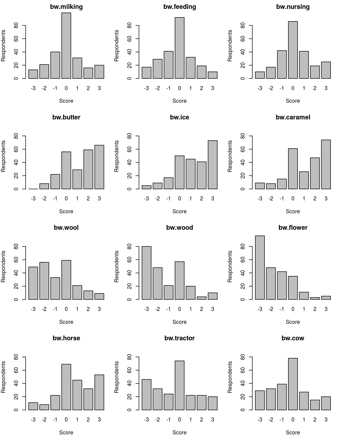
Figure 4.1: Bar plots of BW scores for 12 attribute-levels.
According to the BW scores (BW) or the standardized version (stdBW), the most interesting activity item is butter making (butter); the second most interesting is ice-cream making (ice); and the third most interesting is creamy caramel making (caramel). The BW scores for these three items range from \(284\)–\(307\), and are larger than that for the fourth most interesting activity, horse riding (horse), which has a BW score of 197. The BW scores for the three activities of least interest (i.e., flower, wood, and wool) are \(-394\), \(-299\), and \(-218\), which are all lower than that for tractor riding (tractor), which is the fourth least interesting item. These results indicate that the activity items related to hands-on food processing are relatively popular among the respondents, whereas those related to hands-on craft making are relatively unpopular. This is very useful information for those thinking about developing an agritourism business.
BW scores can be calculated according to groups of respondents. For example, the scores for males and females can be obtained as follows:
##           B   W   BW    stdBW
## milking  62  62    0  0.00000
## feeding  51  78  -27 -0.07500
## nursing  72  56   16  0.04444
## butter  179  23  156  0.43333
## ice     178  32  146  0.40556
## caramel 169  43  126  0.35000
## wool     30 168 -138 -0.38333
## wood     36 173 -137 -0.38056
## flower    4 247 -243 -0.67500
## horse   151  29  122  0.33889
## tractor  83  92   -9 -0.02500
## cow 65 77 -12 -0.03333## B W BW stdBW
## milking 69 67 2 0.005556
## feeding 55 78 -23 -0.063889
## nursing 85 53 32 0.088889
## butter 179 28 151 0.419444
## ice 176 26 150 0.416667
## caramel 180 22 158 0.438889
## wool 49 129 -80 -0.222222
## wood 27 189 -162 -0.450000
## flower 30 181 -151 -0.419444
## horse 121 46 75 0.208333
## tractor 52 143 -91 -0.252778
## cow 57 118 -61 -0.169444Bar plots for respondents in their 20s and those in their 50s can also be drawn using the following lines of code (resultant figures are omitted):
4.9.2 The modeling approach
Finally, we fit the conditional logit model to the Case 2 BWS responses on the basis of the paired, marginal, and marginal sequential models; with both attribute and attribute-level variables. The function clogit() is used to fit the models. Although this function has many arguments, only two are used in this example. The simple call to the function is
with arguments:
formula: A model formula.data: A data frame containing the variables used in the model formula.
The structure of the model formula is similar to that for a linear regression function, lm(): the dependent variable is set on the left-hand side of ~, whereas the independent variables are set on the right-hand side according to a systematic component of the utility function to be fitted. Unlike lm(), however, a stratification variable must be added to the end of the right-hand side of ~ using the strata() function. As shown above, the stratification variable used in clogit() is automatically generated as a variable STR and stored in the dataset created using the function bws2.dataset(). The attribute variable regarding craft making (craft) is omitted from the model. Therefore, the systematic component of the utility function for the example under our model settings is:
\[\begin{align}
v = &\beta_{1}chore + \beta_{2}food + \beta_{3}outdoor + \beta_{4}milking + \beta_{5}feeding + \beta_{6}butter + \beta_{7}ice + \notag \\
&\beta_{8}wool + \beta_{9}wood + \beta_{10}horse + \beta_{11}tractor,
\end{align}\]
where \(chore\), \(food\), and \(outdoor\) are attribute variables; and \(milking\), \(feeding\), \(butter\), \(ice\), \(wool\), \(wood\), \(horse\), and \(tractor\) are attribute-level variables. The model formula for clogit(), corresponding to the systematic component mentioned above, is described (and stored as an object mf) as:
mf <- RES ~ chore + food + outdoor + milking + feeding + butter + ice +
             wool + wood + horse + tractor +
             strata(STR)
After finishing the preparation for the conditional logit model analysis, we fit the model using the clogit() function with the dataset pr.data1 (the paired model):
## Call:
## clogit(formula = mf, data = pr.data1)
##
##           coef exp(coef) se(coef)    z      p
## chore    0.735     2.085    0.042 17.6 <2e-16
## food     1.444     4.237    0.045 32.1 <2e-16
## outdoor  0.758     2.135    0.042 18.1 <2e-16
## milking  0.016     1.016    0.047  0.3    0.7
## feeding -0.169     0.844    0.047 -3.6  4e-04
## butter   0.041     1.042    0.049  0.8    0.4
## ice      0.009     1.009    0.049  0.2    0.9
## wool     0.309     1.362    0.048  6.4  2e-10
## wood     0.024     1.024    0.049  0.5    0.6
## horse    0.629     1.875    0.048 13.1 <2e-16
## tractor -0.363     0.695    0.047 -7.6  2e-14
##
## Likelihood ratio test=1432  on 11 df, p=<2e-16
## n= 25920, number of events= 2160
In this output, the column coef contains the estimated coefficients; column exp(coef) is the exponential function of the estimated coefficients; column se(coef) is the standard error of the estimated coefficients; and columns z and p give the \(z\)-value and \(p\)-value under the null hypothesis, in which the coefficient is zero.
In this example, the estimated coefficients for attribute variables show attribute impact, which is the mean utility across all levels of an attribute (Flynn et al. 2008). The hands-on craft making is the base attribute against which the other attributes are evaluated. The estimated coefficients regarding three attribute variables (i.e., chore, food, and outdoor) are all positive and statistically significant. This means that hands-on craft making is the activity that provides the least attribute impact. Compared with the hands-on craft making, the hands-on food processing has the highest attribute impact, and the hands-on ranch chores and outdoor activities have a similar positive attribute impact.
The attribute-level variables are effect-coded, and thus the coefficient of the base level in each attribute can be calculated using:
b <- coef(pr.out)
nursing <- -sum(b[4:5])
names(nursing) <- "nursing"
caramel <- -sum(b[6:7])
names(caramel) <- "caramel"
flower <- -sum(b[8:9])
names(flower) <- "flower"
cow <- -sum(b[10:11])
names(cow) <- "cow"
craft <- 0
names(craft) <- "craft"
paired.model <- c(b[1:2], craft, b[3], b[4:5], nursing, b[6:7],
   caramel, b[8:9], flower, b[10:11], cow)
par(mai = c(0.05, 0.68, 0.68, 0.35))
x <- barplot(paired.model, axes = FALSE, ylim = c(-1.1, 2), axisnames = FALSE)
axis(2, at = c(0, 0.5, 1, 1.5, 2.0), cex.axis = 0.7)
text(x = x, y = -0.7, labels = names(paired.model), cex = 0.7, srt = 60)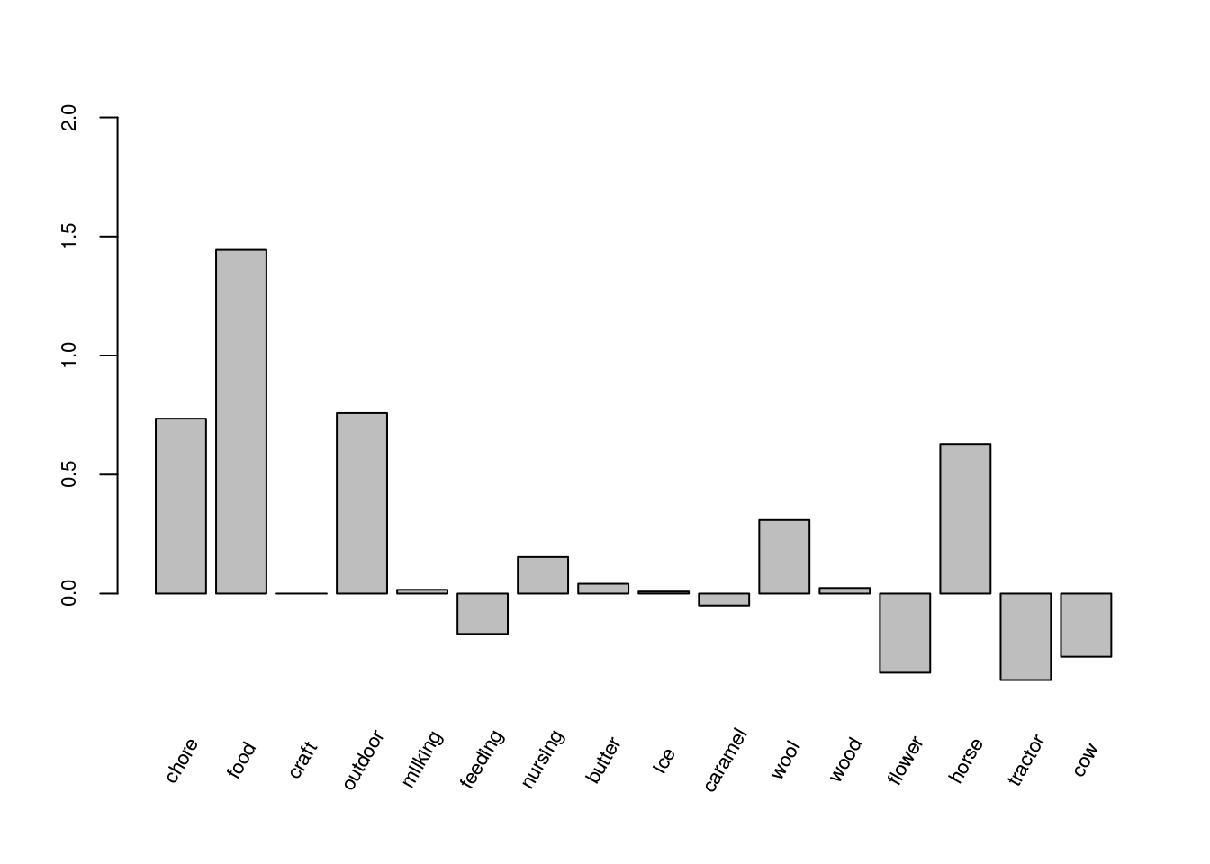
Figure 4.2: Bar plot of the estimated coefficients of the attribute and attribute-level variables for the paired model.
Figure 4.2 shows the estimated coefficients of the attribute and attribute-level variables in the paired model. Comparing the difference between the maximum estimated coefficient for the attribute-level variable and the minimum in each attribute, outdoor has the maximum range and hands-on food making has the minimum range.
The following code is for the marginal model.
## Call:
## clogit(formula = mf, data = mr.data1)
##
##          coef exp(coef) se(coef)    z      p
## chore    0.93      2.53     0.05 19.9 <2e-16
## food     1.83      6.22     0.05 37.6 <2e-16
## outdoor  0.95      2.60     0.05 20.6 <2e-16
## milking  0.02      1.02     0.05  0.4    0.7
## feeding -0.22      0.80     0.05 -4.1  4e-05
## butter   0.05      1.05     0.05  0.9    0.4
## ice      0.01      1.01     0.05  0.2    0.8
## wool     0.37      1.45     0.05  7.0  3e-12
## wood     0.02      1.02     0.05  0.4    0.7
## horse    0.81      2.25     0.05 15.0 <2e-16
## tractor -0.47      0.63     0.05 -8.7 <2e-16
##
## Likelihood ratio test=1862  on 11 df, p=<2e-16
## n= 17280, number of events= 4320
b <- coef(mr.out)
nursing <- -sum(b[4:5])
names(nursing) <- "nursing"
caramel <- -sum(b[6:7])
names(caramel) <- "caramel"
flower <- -sum(b[8:9])
names(flower) <- "flower"
cow <- -sum(b[10:11])
names(cow) <- "cow"
marginal.model <- c(b[1:2], craft, b[3], b[4:5], nursing, b[6:7],
caramel, b[8:9], flower, b[10:11], cow)
par(mai = c(0.05, 0.68, 0.68, 0.35))
x <- barplot(marginal.model, axes = FALSE,
ylim = c(-1.1, 2), axisnames = FALSE)
axis(2, at = c(0, 0.5, 1, 1.5, 2.0), cex.axis = 0.7)
text(x = x, y = -0.7, labels = names(marginal.model), cex = 0.7, srt = 60)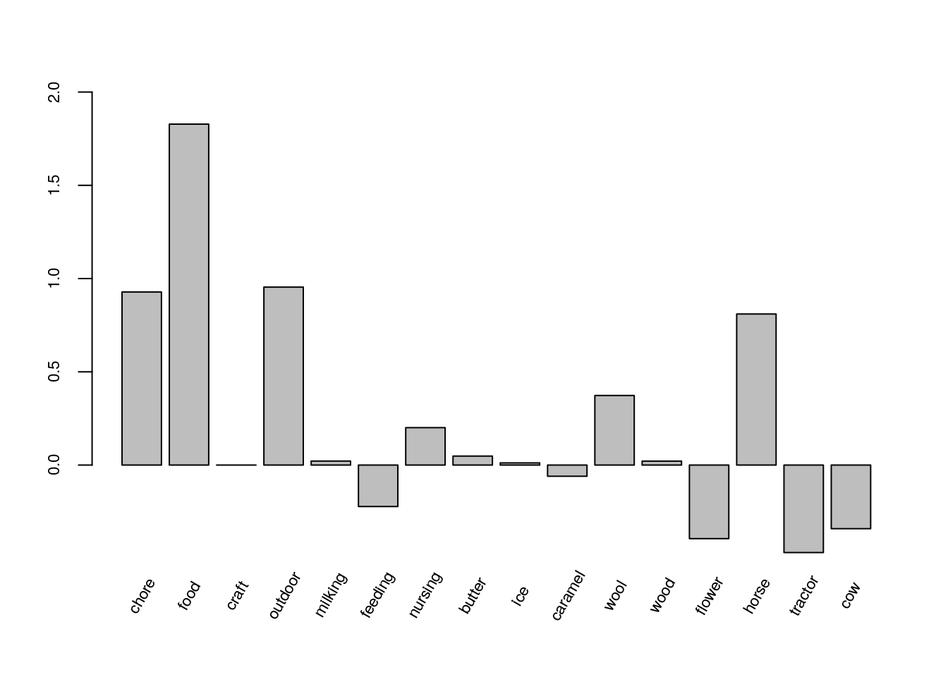
Figure 4.3: Bar plot of the estimated coefficients of the attribute and attribute-level variables for the marginal model.
As expected based on the discussion in Flynn et al. (2008), the estimated coefficients for the attribute and attribute level variables in the marginal model (Figure 4.3) are similar to those in the paired model (Figure 4.2).
The following is for the marginal sequential model.
## Call:
## clogit(formula = mf, data = sq.data1)
##
##           coef exp(coef) se(coef)    z      p
## chore    0.841     2.319    0.047 17.9 <2e-16
## food     1.665     5.283    0.050 33.2 <2e-16
## outdoor  0.839     2.314    0.048 17.6 <2e-16
## milking  0.023     1.023    0.054  0.4    0.7
## feeding -0.196     0.822    0.054 -3.6  3e-04
## butter   0.051     1.052    0.056  0.9    0.4
## ice      0.007     1.007    0.056  0.1    0.9
## wool     0.342     1.408    0.055  6.3  4e-10
## wood     0.005     1.005    0.055  0.1    0.9
## horse    0.751     2.120    0.055 13.6 <2e-16
## tractor -0.459     0.632    0.055 -8.3 <2e-16
##
## Likelihood ratio test=1428  on 11 df, p=<2e-16
## n= 15120, number of events= 4320
b <- coef(sq.out)
nursing <- -sum(b[4:5])
names(nursing) <- "nursing"
caramel <- -sum(b[6:7])
names(caramel) <- "caramel"
flower <- -sum(b[8:9])
names(flower) <- "flower"
cow <- -sum(b[10:11])
names(cow) <- "cow"
marginal.sequential.model <- c(b[1:2], craft, b[3], b[4:5], nursing, b[6:7],
caramel, b[8:9], flower, b[10:11], cow)
par(mai = c(0.05, 0.68, 0.68, 0.35))
x <- barplot(marginal.sequential.model, axes = FALSE,
ylim = c(-1.1, 2), axisnames = FALSE)
axis(2, at = c(0, 0.5, 1, 1.5, 2.0), cex.axis = 0.7)
text(x = x, y = -0.7, labels = names(marginal.sequential.model),
cex = 0.7, srt = 60)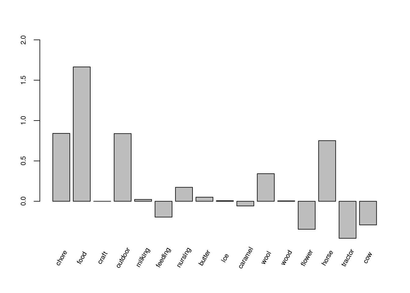
Figure 4.4: Bar plot of the estimated coefficients of the attribute and attribute-level variables for the marginal sequential model.
The estimated coefficients for the attribute and attribute level variables in the marginal sequential model (Figure 4.4) are also similar to those in the paired model (Figure 4.2).
Appendix 4A: Using the mlogit package
The function mlogit.data() in the mlogit package converts a dataset prepared for clogit() into a dataset that can be used with mlogit():
library(mlogit)
mlogit.pr.data1 <- mlogit.data(data = pr.data1,
                               choice = "RES",
                               shape = "long",
                               alt.var = "PAIR",
                               chid.var = "STR",
                               id.var = "id")
mlogit.mr.data1 <- mlogit.data(data = mr.data1,
                               choice = "RES",
                               shape = "long",
                               alt.var = "ALT",
                               chid.var = "STR",
                               id.var = "id")
mlogit.sq.data1 <- mlogit.data(data = sq.data1,
                               choice = "RES",
                               shape = "long",
                               alt.var = "ALT",
                               chid.var = "STR",
                               id.var = "id")
The following lines of code fit the paired, marginal, and marginal sequential models using mlogit().
mf.mlogit <- RES ~ chore + food + outdoor + milking + feeding + butter + ice +
                   wool + wood + horse + tractor - 1
pr.out.mlogit <- mlogit(formula = mf.mlogit, data = mlogit.pr.data1)
mr.out.mlogit <- mlogit(formula = mf.mlogit, data = mlogit.mr.data1)
sq.out.mlogit <- mlogit(formula = mf.mlogit, data = mlogit.sq.data1)
coef(pr.out.mlogit)
## chore food outdoor milking feeding butter ice wool
## 0.734854 1.443925 0.758313 0.015845 -0.169491 0.041439 0.008655 0.308927
## wood horse tractor
## 0.023587 0.628761 -0.363275## chore food outdoor milking feeding butter ice wool
## 0.92798 1.82811 0.95424 0.02153 -0.22215 0.04816 0.01181 0.37304
## wood horse tractor
## 0.02133 0.81006 -0.46898## chore food outdoor milking feeding butter ice wool
## 0.841138 1.664508 0.838893 0.022857 -0.196094 0.050784 0.006766 0.341893
## wood horse tractor
## 0.004922 0.751331 -0.458687References
Aizaki, H. 2019a. Support.BWS2: Tools for Case 2 Best-Worst Scaling. https://CRAN.R-project.org/package=support.BWS2.
Aizaki, H., and J. Fogarty. 2019. “An R Package and Tutorial for Case 2 Best–Worst Scaling.” Journal of Choice Modelling 32: 100171. https://doi.org/10.1016/j.jocm.2019.100171.
Al-Janabi, H., T. N. Flynn, and J. Coast. 2011. “Estimation of a Preference-Based Carer Experience Scale.” Medical Decision Making 31 (3): 458–68. https://doi.org/10.1177/0272989X10381280.
Croissant, Y. 2020b. “Estimation of Random Utility Models in R: The Mlogit Package.” Journal of Statistical Software 95 (11): 1–41. https://doi.org/10.18637/jss.v095.i11.
Flynn, T. N., J. J. Louviere, T. J. Peters, and J. Coast. 2007. “Best–Worst Scaling: What It Can Do for Health Care Research and How to Do It.” Journal of Health Economics 26 (1): 171–89. https://doi.org/10.1016/j.jhealeco.2006.04.002.
Flynn, T. 2008. “Estimating Preferences for a Dermatology Consultation Using Best–Worst Scaling: Comparison of Various Methods of Analysis.” BMC Medical Research Methodology 8 (1): 76. https://doi.org/10.1186/1471-2288-8-76.
Groemping, U. 2020. CRAN Task View: Design of Experiments (DoE) & Analysis of Experimental Data. https://CRAN.R-project.org/view=ExperimentalDesign.
Grömping, U. 2018. “R Package DoE.base for Factorial Experiments.” Journal of Statistical Software 85 (5): 1–41. https://doi.org/10.18637/jss.v085.i05.
Hensher, D. A., J. M. Rose, and W. H. Greene. 2015. Applied Choice Analysis. 2nd ed. Cambridge, UK: Cambridge University Press.
Louviere, J. J., T. N. Flynn, and A. A. J. Marley. 2015. Best–Worst Scaling: Theory, Methods and Applications. Cambridge, UK: Cambridge University Press.
Marley, A. A. J., T. N. Flynn, and J. J. Louviere. 2008. “Probabilistic Models of Set-Dependent and Attribute-Level Best–Worst Choice.” Journal of Mathematical Psychology 52 (5): 281–96. https://doi.org/10.1016/j.jmp.2008.02.002.
R Core Team. 2021a. An Introduction to R. https://CRAN.R-project.org/manuals.html.
R Core Team. 2021b. R: A Language and Environment for Statistical Computing. Vienna, Austria: R Foundation for Statistical Computing. https://www.R-project.org/.
Sarrias, M., and R. Daziano. 2017. “Multinomial Logit Models with Continuous and Discrete Individual Heterogeneity in R: The Gmnl Package.” Journal of Statistical Software, Articles 79 (2): 1–46. https://doi.org/10.18637/jss.v079.i02.
Therneau, T. M. 2020. Survival: Survival Analysis. https://CRAN.R-project.org/package=survival.
Zeileis, A. 2020. CRAN Task View: Econometrics. https://CRAN.R-project.org/view=Econometrics.