Chapter 1 An Illustrative Example of Contingent Valuation

Authors: James Fogarty and Hideo Aizaki

Latest Revision: 29 August 2019 (First Release: 30 March 2018)

1.1 Before you get started

Most of the steps involved in the analysis of contingent valuation (CV) data are fully explained in this guide; however, the explanations assume some familiarity with R (R Core Team 2021b)/RStudio Desktop (RStudio 2020). If you are completely unfamiliar with these software platforms, you are advised to consult Introduction to R (R Core Team 2021a) and other general support material before working through these examples. The work is derived from teaching materials originally written by James Fogarty.

1.2 Overview

The Contingent Valuation (CV) method is widely used to obtain estimates of the value of goods and services where there is no `market’ price. As a practical matter, a typically question of interest for a CV study is something like: Would you be willing to pay $25, annually, to reduce local air pollution by 50 percent?, where the answer to the question is either yes or no. We call this question format a single-bounded dichotomous choice (SBDC) survey question. Frequently, after asking an initial question in the SBDC format, respondents are asked to answer an additional (follow-up) question that has the same structure as the original willing to pay question but uses a different dollar value. For example, if a survey respondent answered yes, they were willing to pay $25 to the survey question on air pollution they might then be asked as the follow-up question: Would you be willing to pay $50, annually, to reduce local air pollution by 50 percent?. If the respondent had answered no, they are not willing to pay $25 to reduce air pollution, the follow-up question might then be: : Would you be willing to pay $10, annually, to reduce local air pollution by 50 percent?.

When a follow-up willingness is known as a double-bounded dichotomous choice (DBDC) format. This guide focuses on only SBDC and DBDC CV studies.

From the answers to the ‘willingness to pay’ (WTP) question, the objective is to find either the mean or the median WTP for the proposed change. Although both the mean and the median are valid measure of central tendency, the convention in most studies has been to look at the median WTP. The median WTP has an interpretation as the price that would be supported by half the population, and so is the value that has majority community support. There are also a range of technical issues that need to be addressed when calculating the mean WTP that complicate the analysis. As such, here we generally focus on the median WTP estimate.

For statistical analysis, the ‘yes’/‘no’ data we get from the answers to the WTP survey question is usually coded as ‘yes’ = 1, ‘no’ = 0, and so the response variable is a dichotomous [0, 1] variable. This means that the general tools of statistical analysis used for [0, 1] data are used for CV analysis. However, the general tools for binary data are not available to analyze DBDC-CV data.

Although there are several R packages that can be used to analyze CV data, this guide explains how to use the DCchoice package (Nakatani, Aizaki, and Sato 2020) distributed from the Comprehenshive R Archive Network (CRAN). The DCchoice package has: (i) been created specifically for CV analysis; (ii) includes a range of additional features that add value to CV studies, such as the ability to estimate non-parametric models; and (iii) is (relatively) easy to use. As such, this guide focuses on how to undertake a structured CV studies using the DCchoice package.

The focus of the guide is on the practical skills needed to undertake a primary CV study using industry standard methods. The guide does not cover the theory behind the models presented, and nor does it cover some alternative very useful approaches, such as non-parametric methods. The guide does, however, provide the reader with the tools necessary to estimate WTP from a primary CV study. For the theoretical and/or detailed explanation of both SBDC and DBDC contingent valuation models please refer to works such as Bateman and Willis (1999), Bateman et al. (2002), and Carson and Hanemann (2005). For the details of the DCchoice package please see Aizaki, Nakatani, and Sato (2014) .

1.3 Getting started with contingent valuation analysis

Once you have R open, to follow this example you need to install and load three additional packages DCchoice, Ecdat (Croissant and Graves 2020) and lmtest (Zeileis and Hothorn 2002). If you are unsure of how to install a package please consult the relevant reference material on How to install R packages.

Although Ecdat and lmtest can be installed into your R installation in the standard manner used for installing packages from CRAN, you may need to follow a different method to install DCchoice. This is because DCchoice depends on a package distributed from the Bioconductor repository. As such, to install DCchocie it is recommended that you copy and execute the following code chunk in your R console:

install.packages("DCchoice",
  repos = c("http://www.bioconductor.org/packages/release/bioc",
            "https://cran.rstudio.com/"),
  dep = TRUE)

Once the relevant packages have been installed, the next step is to load the DCchioce, Ecdat and lmtest packages for your current session. The DCchioce package contains the main functions that we will use for the analysis, but we also need some of the functions available in the lmtest package. The Ecdat package contains real world data sets that have been made publicly available, and for this example we will be using the NaturalParks data set to illustate how CV study data can be analysised.

library(DCchoice)
library(Ecdat)
library(lmtest)

Note that the following line of code is needed to reproduce the results on R 3.6.0 or later:

if(getRversion() >= "3.6.0") RNGkind(sample.kind = "Rounding")

## Warning in RNGkind(sample.kind = "Rounding"): non-uniform 'Rounding' sampler
## used

Normally you will need to load a data set into R, using a command something like:

myCVdata <- read.csv("source_data_CV_study.csv")

where "source_data_CV_study.csv" is the relevant data file in your working directory. Here, as we are using one of the in-built sample data sets from the Ecdat package, the command is a little different. Once we have loaded the data, we can use the head() function to see what the data looks like. By default the head() function will show the first six rows of data, and the column headings, but you can use the n argument to specify exactly how many rows of data are displayed. The head() function helps you visualise what the data looks like.

data(NaturalPark, package = "Ecdat") # Access the example data file
NP <- NaturalPark                    # Rename the data file to something short
head(NP, n = 3)                      # Display the first three rows of data 

##   bid1 bidh bidl answers age    sex income
## 1    6   18    3      yy   1 female      2
## 2   48  120   24      yn   2   male      1
## 3   48  120   24      yn   2 female      3

The columns of data in the NP (that is, NaturalPark) data set contain the following seven variables:

• bid1: the initial bid amount (in euros) used in the first WTP question. Typically we only have a small number of bid amounts, and here there are four bid amounts: 6, 12, 24 and 48 ;
• bidh: if the respondent answered ‘yes’ to the first question the higher bid amount used for the follow up WTP question;
• bidl: if the respondent answer ‘no’ to the first question the lower bid amount used for the follow up WTP question;
• answers: the coding of the answers to the two questions (nn, ny, yn, yy), y = ‘yes’ and n = ‘no’. Note that variables of this format are called factor variables, and as there are four combinations, we say that the variable has four levels;
• age: rather than report their exact age respondents were asked to identify which age bracket they belong to. There were six age brackets, and in the coding higher numbers are associated with older people;
• sex: is a factor variable with two levels (male, female);
• income: similar to age respondents were not asked their exact income, but were asked which income bracket they were in. There were eight income brackets and higher numbers represent higher income brackets.

In addion to the head() function, whenever you load data into R you should also use the str() function to check the data structure. Sometimes data is not read into R the way you think would have been. In particular, whether or not a data column is coded as a factor variable or not is something that you often need to check. The value of the str() function is that it allows you to see what type of variables you have.

str(NP)   #  Another way to check the data structure 

## 'data.frame':    312 obs. of  7 variables:
##  $ bid1   : int  6 48 48 24 24 12 6 12 24 6 ...
##  $ bidh   : int  18 120 120 48 48 24 18 24 48 18 ...
##  $ bidl   : int  3 24 24 12 12 6 3 6 12 3 ...
##  $ answers: Factor w/ 4 levels "nn","ny","yn",..: 4 3 3 1 2 1 4 3 3 4 ...
##  $ age    : int  1 2 2 5 6 4 2 3 2 3 ...
##  $ sex    : Factor w/ 2 levels "male","female": 2 1 2 2 2 1 2 1 2 1 ...
##  $ income : int  2 1 3 1 2 2 3 2 2 3 ...

For this example we can now see that we have 312 observations, which means we have 312 survey responses, and seven variables. The description of the data also provides information on the type of variable we have in each column, and in this instance we have a mix in integer variables and factor variables.

1.4 The single-bounded dichotomous choice question model

This approach remains one of the most widely seen in the literature, and to work through a SBDC example is also helpful as a benchmark to use for comparisons to a DBDC example.

1.4.1 Data management

The first step in the process is to check that the data have been read in R properly.

Although the data set contains information on a DBDC CV survey, for this first example we use only the information from the first WTP question. That is, we treat the data set as if it were a SBDC CV study. To set up the model for analysis we need a column that contains a 1 if a respondent said ‘yes’ to the first WTP question, and contains a 0 if the respondent said ‘no’ to the first WTP question.

Unless you have a programming background, it is generally easier to manage data in MS Excel rather than directly in R, but it is possible to perform data management functions in R, as is done here. The R code below adds a new column to the dataframe NP called ans1, where the coding is 1 if a respondent said ‘yes’ to the first WTP question and 0 if they said ‘no’.

Data management in R is a bit different to data management in MS Excel. Often you will find it quickest and easiest to create new data columns and edit your data in MS Excel rather than in R. MS Excel is great for data management; so if you are already confortable using MS Excel to manage data files there is no need to learn the data management tricks in R. Here we perform the data management directly in R to ensure reproducibility of the example.

NP$ans1 <- ifelse(NP$answers == "yy" | NP$answers == "yn", 1, 0)

After we have added the new variable to the dataframe, we again use the str() function to check that the variable we created has been attached as expected. Here we see that a new variable ans1, which contains only 1s and 0s has been successfully added as a new column at the end of the dataframe.

str(NP)

## 'data.frame':    312 obs. of  8 variables:
##  $ bid1   : int  6 48 48 24 24 12 6 12 24 6 ...
##  $ bidh   : int  18 120 120 48 48 24 18 24 48 18 ...
##  $ bidl   : int  3 24 24 12 12 6 3 6 12 3 ...
##  $ answers: Factor w/ 4 levels "nn","ny","yn",..: 4 3 3 1 2 1 4 3 3 4 ...
##  $ age    : int  1 2 2 5 6 4 2 3 2 3 ...
##  $ sex    : Factor w/ 2 levels "male","female": 2 1 2 2 2 1 2 1 2 1 ...
##  $ income : int  2 1 3 1 2 2 3 2 2 3 ...
##  $ ans1   : num  1 1 1 0 0 0 1 1 1 1 ...

Typically we implement our survey such that the number of survey responses for each bid value is approximately equal. If we use the table() function we can see the distribution of responses by bid value:

table(NP$ans1, NP$bid1) 

##    
##      6 12 24 48
##   0 26 34 40 41
##   1 50 43 42 36

You read the table information as follows:

• There are 76 survey responses for a bid price of six euro. At a price of €6, of the 76 responses, 50 people said yes they would be willing to pay €6 and 26 said no they would not be willing to pay €6.

• There are 77 observations for a bid price of 12 euro. At price of €12, of the 77 responses, 43 people said yes they would be willing to pay €12 and 34 said no they would not be willing to pay €12.

• Etc.

As the bid price increases, we expect that a smaller proportion of people will say ‘yes’ they are willing to pay the amount to achieve, say, a fixed environmental improvement. This basic pattern can be seen in the table by reading across the ‘1’ row, which shows the number of ‘yes’ respondents falling from \(50\) to \(36\).

1.4.2 Data visualisation

The second step in the process is to look at the data visually. Whenever we perform a statistical test there is the possibility of making either a Type I error or a Type II error. The possibility of making a Type I error increase with the number of tests we conduct; so, if we can learn something about the data structure without needing to rely on a statistical test that is valuable.

Although the number of observations for each bid value is approximately equal, as we code responses as yes = 1 and no = 0, the easiest way to see if the ‘proportion’ of people saying yes falls as the bid price increases is to calculate the group mean for each bid level. It is easy to calculate group mean information in MS Excel, but here we use the tapply() function to calculate the group means, and to keep the reporting of results simple we apply the round() function to the results to limit reporting to two decimal places.

round(tapply(NP$ans1, NP$bid1, mean), 2)

##    6   12   24   48 
## 0.66 0.56 0.51 0.47

From the group mean information it can be seen that as the bid price increases, the proportion of people that are willing to pay each amount falls. This is what we expect, and in the economics literature this relationship is known as the law of demand.

It is also possible to plot this information. Figure 1.1 show two examples of a relevant plot. The plot on the left is a minimal basic example of the kind we would use to develop our own understanding of the data. This kind of plot is OK when you want to just quickly look at the data. The plot on the right illustrates some useful R plotting features, and is closer to the kind of plot needed for a research report.

# A basic barplot
barplot(tapply(NP$ans1, NP$bid1, mean)) 

# More advanced barplot suitable for a research report
with(NP, barplot(round(tapply(ans1, bid1, mean), 2), las = 1,
         xlab = "Bid value categories in euros", 
         ylab = "Proportion of selecting yes", 
         yaxs = 'i', xaxs = 'i', 
         main = "Implied demand 'curve'",
         border = NA, font.main = 4))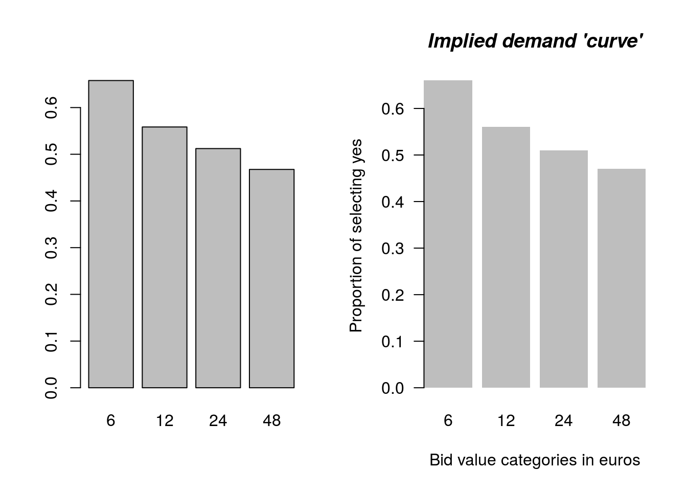

Figure 1.1: Basic and custom plot

Looking at a data plot is a key element in the research process, and you should always undertake some simple data visualisation as part of your analysis.

1.4.3 Model estimation

1.4.3.1 A simple model to illustate the estimation process

Let us first fit a very simple model to the data. For the moment we will ignore the information we have on gender, income, and age. The model we fit say that the response value we observe (which is either a ‘0’ for a response of ‘no’, I am not willing to pay this amount, or a ‘1’ for a response of ‘yes’, I am willing to pay this amount) can be explained by the bid value. So we have a model with only one explanatory variable: the bid amount or ‘price’.

Using DCchoice the formula for this type of model is as follows:

mod.out <- sbchoice(dep var ~ exp var | bid, dist = "", data = my.data)

• mod.out: the ‘object’ name that we will save our results to, for our first model we will use sb1 to denote the object that we save results to;
• <-: the assignment operator;
• sbchoice: the function used for model estimation;
• dep var: the model dependent variable (the ‘yes’ and ‘no’ responses coded as 1s and 0s), which for our first model is the variable ans1;
• exp var: this is where we list all the model explanatory variables other than the bid amount. We have no explanatory variables for the first model, just the intercept term, so we have just the ‘1’ term for the intercept ~ 1;
• | bid: this is where we specifiy the bid amount variable. For our example the bid amount variable is bid1;
• dist = "": it is possible to specify different distributions, but we will always use the logistic distribution so this will always read dist = "logistic";
• data = my.data: directions to the appropriate dataframe, which in our case is data = NP.

Following model estimation we generally use the summary() function to look at the results. The summary function provides a lot of information, so first, let’s just look at the coefficent estimates using the coeftest() function which is available from the lmtest package.

# A very simple model
sb1 <- sbchoice(ans1 ~ 1 | bid1,  dist = "logistic", data = NP)
coeftest(sb1)

## 
## z test of coefficients:
## 
##               Estimate Std. Error z value Pr(>|z|)   
## (Intercept)  0.5500450  0.1998739  2.7520 0.005924 **
## BID         -0.0157223  0.0071807 -2.1895 0.028560 * 
## ---
## Signif. codes:  0 '***' 0.001 '**' 0.01 '*' 0.05 '.' 0.1 ' ' 1

The key point to note in the coefficients information is the negative sign on the bid variable. Regardless of the coding in the source file this will always appear as BID in the output summary. The BID coefficent says, as expected, that as the bid price increases, the proportion of people saying ‘yes’ they are willing to pay that amount falls. Further, it can also be seen from the other information in the coefficent table that the finding is ‘statistically significant’.

It is also possible to visualise the model results using the plot() function. Here, in addition to the raw WTP information we add a horizontal line to the plot to highlight the point of 50 percent support. As can be seen from Figure 1.2, the price that has 50 percent support is around €35.

plot(sb1, las = 1)  # plots the predicted support at each bid value 
                    #  las control axis orientation
abline(h = 0.5, lty = 2, col = "red") # adds a horizontal line to the plot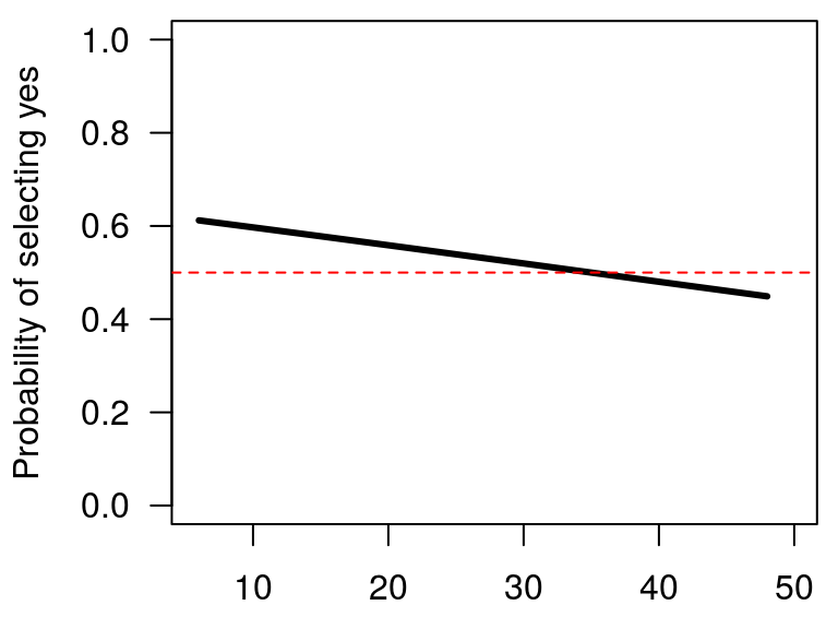 

Figure 1.2: Relationship between WTP and bid price

We now look at the full model summary output we get when we use the sbchoice() function:

summary(sb1)  #  the complete model summary

## 
## Call:
## sbchoice(formula = ans1 ~ 1 | bid1, data = NP, dist = "logistic")
## 
## Formula:
## ans1 ~ 1 | bid1
## 
## Coefficients: 
##              Estimate Std. Error z value Pr(>|z|)   
## (Intercept)  0.550045   0.199874   2.752  0.00592 **
## BID         -0.015722   0.007181  -2.190  0.02856 * 
## ---
## Signif. codes:  0 '***' 0.001 '**' 0.01 '*' 0.05 '.' 0.1 ' ' 1
## 
## Distribution: logistic 
## Number of Obs.: 312  
## log-likelihood: -212.3968 
## pseudo-R^2: 0.0113 , adjusted pseudo-R^2: 0.0020 
## LR statistic: 4.841 on 1 DF, p-value: 0.028 
## AIC: 428.793653 , BIC: 436.279659 
## 
## Iterations: 4  
## Convergence: TRUE 
## 
## WTP estimates:
##  Mean : 63.95526 
##  Mean : 26.04338 (truncated at the maximum bid)
##  Mean : 47.26755 (truncated at the maximum bid with adjustment)
##  Median : 34.98512

The summary output can be read in several parts:

• the first block of information reports back the model that was estimated;
• the second block of information reports the estimated model coefficents — and whether or not the coefficent estimates are ‘statistically significant’ — which we have already looked at;
• the third block of information reports the estimated model fit metrics. These metrics can be used to compared different model specifications, and it is also the convention to report some of this information in report results tables. Note that the line Convergence: TRUE is important. This result tells us that the estimated model did actually solve. If the model does not solve you will see an error message;
• the fourth block of information reports the estimated mean and median WTP. Note that there are three values reported for the mean WTP. Rather than focus on the different estimates of the mean WTP, we will just focus on the median WTP which is €34.99.

Although we now have an ‘estimate’ of the median WTP (for the question we asked), it is important to also report how ‘certain’ we are about this estimate. The question of estimate uncertainty is addressed through calculating confidence intervals for the WTP estimate.

Many methods can be used to calculate approximate confidence intervals for WTP estimates in CV studies, and while each approach has strengths and weaknesses, the different approaches all generally give similar results (Hole 2007). Within DCchoice two methods are available for calculating confidence intervals for the WTP estimate: the bootstap method (Efron and Tibshirani 1993), which is available via the bootCI() function, and the Krinsky Robb method (Krinsky and Robb 1986, 1990), available via the krCI() function. Conceptually, the difference between the two appoaches is that the bootstrap method relies on the sample data distribution when working through the simulation steps while the Krinsky Robb method relies on a theoretical distribution for the simulations. When conducting simulations the results vary (slightly) from simulation to simulation. The differences are trivial in practice, but it is good practice to set a start value (random seed value) for each simulation before you start. If you provide information on the start value for the simulation then it is possible for other to reproduce the same exact result in the future. In R, the way that you set the simulation start value is with the set.seed() function.

Here we want to get confidence intervals for the model sb1. For both the bootstrap method and the Krinsky Robb method it is possible to obtain confidence intervals for any range, but the default setting provides 95 percent confidence intervals (95% CI), and this is the range that is typically reported.

The first simulation we run is for the Krinsky Robb method and the second simulation is for the bootstrap method. Note that it can take a little while for the simulations to run. Although we get information on all four meaures of WTP, we will coninue to focus just on the median WTP estimate.

set.seed(123) # The start value can be anything
krCI(sb1)     # The command to get the relevant 95% CI

## the Krinsky and Robb simulated confidence intervals
##                         Estimate     LB      UB
## Mean                      63.955 40.045 257.703
## truncated Mean            26.043 23.335  28.663
## adjusted truncated Mean   47.268 37.109  62.480
## Median                    34.985 17.722  86.696

set.seed(123) # As it is a new simulation we again set a start value 
bootCI(sb1)   # The command to get the relevant 95% CI

## the bootstrap confidence intervals
##                         Estimate     LB      UB
## Mean                      63.955 37.395 271.494
## truncated Mean            26.043 23.487  28.845
## adjusted truncated Mean   47.268 36.284  63.787
## Median                    34.985 20.697  99.584

The confidence intervals around the median WTP estimate for the two methods are as follows:

• For the Krinsky Robb method the 95% CI is €17.72 to €86.70.
• For the Bootstrap method the 95% CI is € 20.70 to €99.58.

So, while we have a point estimate of €34.99 as the median WTP, from the 95% CI information it can be seen that there is considerable uncertainty surounding this estimate.

Use of a follow up question allows us to reduce WTP estimate uncertainty substantially; but before we go on to estimate the DBDC model, let us first incorporate the additional information we have on age, gender, and income. If we think that there may be a relationship between these variables and someone’s WTP then we should include these variables in the model.

1.4.4 A typical initial model for a single bounded question study

Here we continue with the SBDC model, but we work through the process in a way that is more consistent with the typical modelling approach, which is usually termed a general to specific approach.

In practice, a general to specific modelling approach means that the first model we consider has the largest number of explanatory variables. If some of the explanatory variables in the general model are not statistically significant, depending on the circustance, we may choose to remove these variables from the model and ‘simplify’ the model to make it smaller. However, just because a variable is not statistically significant does not mean that we auotomatically delete the variable from the model. There can be many good reasons to keep a variable in the model even though the variable is not statistically significant.

So, first we specifiy the full model and look at the output. Again, as the first step, we focus on the model coefficents table.

# A relatively complete model
sb.full <- sbchoice(ans1 ~ 1 + age + sex + income | bid1, dist = "logistic", 
    data = NP)
coeftest(sb.full)

## 
## z test of coefficients:
## 
##               Estimate Std. Error z value  Pr(>|z|)    
## (Intercept)  1.4828932  0.4832647  3.0685  0.002151 ** 
## age         -0.3683775  0.0851072 -4.3284 1.502e-05 ***
## sexfemale   -0.6029514  0.2498631 -2.4131  0.015816 *  
## income       0.2536352  0.1054709  2.4048  0.016182 *  
## BID         -0.0195099  0.0077154 -2.5287  0.011449 *  
## ---
## Signif. codes:  0 '***' 0.001 '**' 0.01 '*' 0.05 '.' 0.1 ' ' 1

The first thing to note about the results is that all the variables we have included in the model are statistically significant. This means that in addition to the bid price: age, income, and gender are all variables that help explain whether or not a person said ‘yes’ to the WTP question.

When trying to understand the coefficent estimates, it is useful to focus on the sign of the variable rather than the point estimate. So, here we can say that:

• older people are willing to pay less
• females (coded as female equals one) are willing to pay less
• those with higher incomes are willing to pay more.

Here we plot the relevant information for the two models (Figure 1.3). If you are not yet familar with plotting in R the below example may appear confusing, however if you spend some time looking at the code you might be able to work what each line of code is doing.

# A detailed plot for the simple model
plot(sb1, las = 1, xlab = "Bid amounts in euro", main = "Simple model", 
    cex.main = 0.8, font.main = 4)  # plots  predicted support at each price 
abline(h = 0.5, lty = 2, col = "red")  # adds a horizontal line to the plot 
segments(x0 = 34.99, y0 = -1, x1 = 34.99, y1 = 0.5, col = "red", 
    lty = 2)
points(34.99, 0.5, col = "red", pch = 16)
text(5, 1, "Median WTP estimate = 34.99 euro", pos = 4, cex = 0.7)

# A detailed plot for the full model
plot(sb.full, las = 1, xlab = "Bid amounts in euro", main = "Full model", 
    cex.main = 0.8, font.main = 4)  # plots  predicted support at each price 
abline(h = 0.5, lty = 2, col = "green")  # adds a horizontal line  
segments(x0 = 34.29, y0 = -1, x1 = 34.29, y1 = 0.5, col = "green", 
    lty = 2)
points(34.29, 0.5, col = "green", pch = 16)
text(5, 1, "Median WTP estimate = 34.29 euro", pos = 4, cex = 0.7)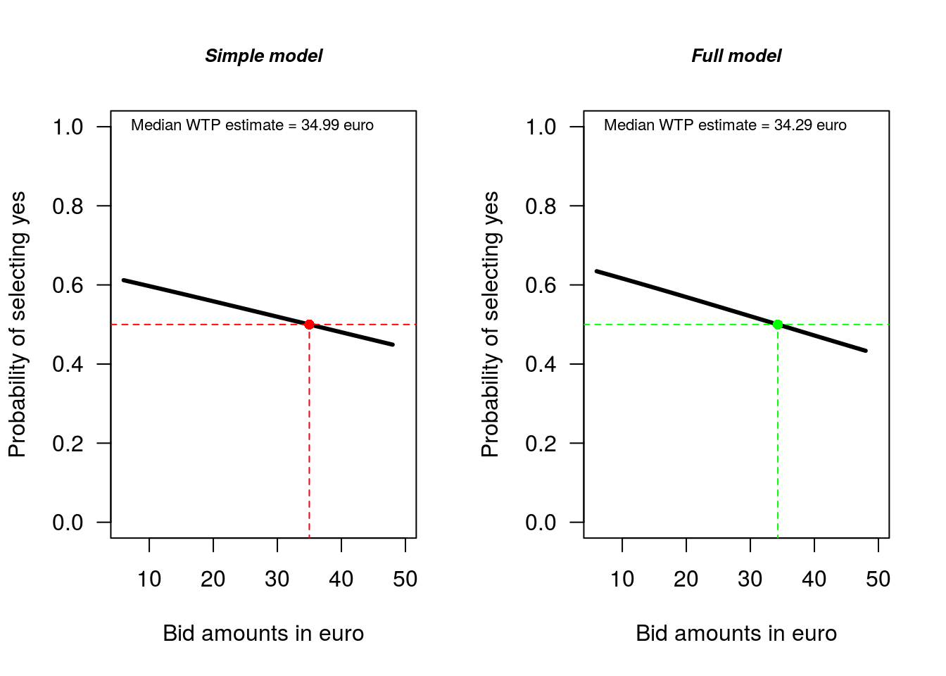

Figure 1.3: Comparison of simple and full model WTP estimates

Although we have already looked at the coefficent results, the main thing we are interested in from a policy perspective is the WTP estimate. We now look at the full model results using the summary function:

summary(sb.full)

## 
## Call:
## sbchoice(formula = ans1 ~ 1 + age + sex + income | bid1, data = NP, dist = "logistic")
## 
## Formula:
## ans1 ~ 1 + age + sex + income | bid1
## 
## Coefficients: 
##              Estimate Std. Error z value Pr(>|z|)    
## (Intercept)  1.482893   0.483265   3.068  0.00215 ** 
## age         -0.368378   0.085107  -4.328  1.5e-05 ***
## sexfemale   -0.602951   0.249863  -2.413  0.01582 *  
## income       0.253635   0.105471   2.405  0.01618 *  
## BID         -0.019510   0.007715  -2.529  0.01145 *  
## ---
## Signif. codes:  0 '***' 0.001 '**' 0.01 '*' 0.05 '.' 0.1 ' ' 1
## 
## Distribution: logistic 
## Number of Obs.: 312  
## log-likelihood: -191.2161 
## pseudo-R^2: 0.1099 , adjusted pseudo-R^2: 0.0866 
## LR statistic: 47.203 on 4 DF, p-value: 0.000 
## AIC: 392.432129 , BIC: 411.147145 
## 
## Iterations: 4  
## Convergence: TRUE 
## 
## WTP estimates:
##  Mean : 55.48958 
##  Mean : 26.35888 (truncated at the maximum bid)
##  Mean : 46.53209 (truncated at the maximum bid with adjustment)
##  Median : 34.2916

Note that compared to the simple model the various measures of model fit for the full model have improved. Given the variables we added to the model are individually statistically significant, it should be the case that the model fit improves.

In terms of the median WTP estimate, there is little difference between the simple (and incorrect) model and the more general model, with median WTP for the simple model €34.99, and median WTP for the full model with additional explanatory variables €34.29. When we have a representative data sample, such outcomes are not uncommon. However as we are interested in understanding the varibles that determine WTP, even if we have a representative sample it is important to consider a model with explanatory variables.

The final step in the analysis is to again establish the 95 percent confidence interval for the median WTP estimate. Here, and in subsequent applications, we will just rely on the bootstrap method to generate the 95% CI. You can use any method, but the bootstrap method is widely understood and so it is the bootstrap method that we use here.

set.seed(123) # We still need a start value for the simulation  
bootCI(sb.full) 

## the bootstrap confidence intervals
##                         Estimate     LB      UB
## Mean                      55.490 35.037 173.200
## truncated Mean            26.359 23.510  29.687
## adjusted truncated Mean   46.532 35.130  64.452
## Median                    34.292 21.891  78.977

As we have a more complete model there is less uncertainty about the WTP estimate. So, even though the median WTP estimates are similar for the simple model and the full model, there is real practical value from having a complete model specification: smaller 95% confidence intervals around the median WTP estimate. Note, however, that the 95% CI still covers a considerable range: €21.89 to €78.98.

One of the most effective ways to redue the level of uncertainty regarding how much people are willing to pay is to ask a follow up question. We now consider this scenario.

1.5 The double-bounded dichotomous choice or follow up question model

To undertake a survey involves considerable cost. If the survey is to be undertaken via a university, the process will involve ethics approval, considerable staff time, and potentially subsantial direct costs. In the private sector the direct financial cost of a survey will almost always be high; as can be the indirect cost of staff time. As direct and indirect survey costs are high — whether in the private sector or the public sector — when conducting a survey it is important to obtain as much information as possible from survey respondents.

When conducting a survey one way to get valuable additional information, at low cost, is to ask a follow up question. For example, say respondents say ‘yes’, they are willing to pay $10 to achieve a specified environmental improvement. At this point all we know is that they are willing to pay at least $10. We have no upper bound estimate of their WTP. All we know about their WTP is that it lies between $10 and \(\infty\). If we then ask the respondents a follow up question, such as are they willing to pay $20, and the respondent says ‘yes’, we have gained some information: they are willing to pay at least $20, but if the respondents say ‘no’, we know that their WTP is between $10 and $20, which is a relatively tight range. The situation is similar for initial responses that are ‘no’, where the next question uses a lower bid amount.

Regardless of the initial response, if we ask a follow up question we get valuable additional information that can help us shrink the 95% CI around the median WTP estimate. With DCchoice it is relatively easy to make use of this additional information. As a practical matter, when we use a DBDC question format we reduce estimate uncertainty, so the 95% CI around the median WTP estimate will become smaller.

1.5.1 Data management for the double bounded question

Before we estimate the DBDC model we need to perform some further data management. Specifically, we need to: (i) add a a new column to the dataframe that contains a 1 if the respondent said ‘yes’ to the second WTP question and 0 if the respondent said ‘no’; and (ii) add a column that contains the second bid value. Note that the second bid value depends on the response to the first question. If the survey respondent said ‘yes’ to the first WTP question, the bid amount increased for the second question; and if the survey respondent said ‘no’ to the first WTP question, the bid amount goes down. Note that it is also possible to perform data management in MS Excel. Here the data management is done in R to ensure reproducibility.

# Note data management can also be done in MS Excel
NP$ans2 <- ifelse(NP$answers == "yy" | NP$answers == "ny", 1, 0)
NP$bid2 <- ifelse(NP$ans1 == 1,  NP$bidh, NP$bidl)

Whenever you add new variables to a dataframe it is necessay to check the variables have been added correctly. Typically you will use the str() function to do this, but you can also check the data structure with the head() function.

head(NP, n = 10)

##    bid1 bidh bidl answers age    sex income ans1 ans2 bid2
## 1     6   18    3      yy   1 female      2    1    1   18
## 2    48  120   24      yn   2   male      1    1    0  120
## 3    48  120   24      yn   2 female      3    1    0  120
## 4    24   48   12      nn   5 female      1    0    0   12
## 5    24   48   12      ny   6 female      2    0    1   12
## 6    12   24    6      nn   4   male      2    0    0    6
## 7     6   18    3      yy   2 female      3    1    1   18
## 8    12   24    6      yn   3   male      2    1    0   24
## 9    24   48   12      yn   2 female      2    1    0   48
## 10    6   18    3      yy   3   male      3    1    1   18

If you look at the first row of the data and the bid1 column, it can be seen that the first respondent in the dataset was asked if they would be willing to pay €6 for the first question. From the answers column it can be seen that the respondent said ‘yes’ to this question and so in the ans1 column there is a 1. As the respondent said ‘yes’ to the first WTP question, the bid amount for the second question increases to €18, which is the value recorded in the bid2 column. As the respondent also said ‘yes’ to this question, there is a 1 in the ans2 column.

Read through some of the other rows of the dataframe to make sure that you can follow the coding. Also note the patern for the bid amounts. There are four possible initial bid values: €6, €12, €24, and €48, and the second bid amount have the following pattern:

• If the first bid value is €6 and the answer is ‘yes’, the second bid value increases to €18, and if the answer is ‘no’ the second bid value decreases to €3;
• If the first bid value is €12 and the answer is ‘yes’, the second bid value increases to €24, and if the answer is ‘no’ the second bid value decreases to €6;
• If the first bid value is €24 and the answer is ‘yes’, the second bid value increases to €48, and if the answer is ‘no’ the second bid value decreases to €12;
• If the first bid value is €48 and the answer is ‘yes’, the second bid value increases to €120, and if the answer is ‘no’ the second bid value decreases to €24.

1.5.2 An initial general double bounded model

Similar to the approach taken for the SBDC model we start with a general model and then look at the results via the summary() function.

Using DCchoice the general formula for a DBDC model is as follows:

db.out <- dbchoice(dep var1 + dep var2 ~ exp var | bid1 + bid2, dist = "", data = mydata)

• db.out: this is the ‘object’ that we will save our results to;
• <-: the assignment operator;
• dbchoice: the function used for model estimation;
• dep var1 + dep var: the model dependent variables (the ‘yes’ and ‘no’ responses coded as 1s and 0s for each question);
• ~ exp var: this is where we list all the model explanatory variables other than the bid amount;
• | bid1 + bid2: this is where we specifiy the bid amount variables for question 1 and question 2;
• dist = "logistic": we will always use the logistic;
• data = mydata: directions to the appropriate dataframe.

db.full <- dbchoice(ans1 + ans2 ~ 1 + age + sex + income | bid1 + bid2, dist = "logistic", 
    data = NP)
coeftest(db.full)

## 
## z test of coefficients:
## 
##               Estimate Std. Error  z value  Pr(>|z|)    
## (Intercept)  1.4219530  0.3919483   3.6279 0.0002857 ***
## age         -0.3253981  0.0756503  -4.3013 1.698e-05 ***
## sexfemale   -0.2560669  0.2162875  -1.1839 0.2364451    
## income       0.2451780  0.0884177   2.7730 0.0055550 ** 
## BID         -0.0500067  0.0041104 -12.1660 < 2.2e-16 ***
## ---
## Signif. codes:  0 '***' 0.001 '**' 0.01 '*' 0.05 '.' 0.1 ' ' 1

Looking at the coefficents table it can be seen that the results for the DBDC model are similar to those for the SBDC model, but there are some important differences. For example, in the DBDC model gender is no longer statistically significant.

Also note the difference in the size of the z value assocaited with the BID variable between the SBDC question and the DBDC question. With the DBDC question the z value has become larger, which means that we have been able to estimate the price effect more precisely.

In this instance, although the gender effect is not statistically significant, we are going to leave the variable in the model. There is considerable published research showing that gender does have an effect on WTP estimates, and because of this we are going to leave the gender variable in the model.

If we look at the full summary output, and the median WTP value, we can see that the estimate from the DBDC model is around half the value reported for the SBDC model.

summary(db.full)

## 
## Call:
## dbchoice(formula = ans1 + ans2 ~ 1 + age + sex + income | bid1 + bid2, 
##     data = NP, dist = "logistic")
## 
## Formula:
## ans1 + ans2 ~ 1 + age + sex + income | bid1 + bid2
## 
## Coefficients: 
##             Estimate Std. Error z value  Pr(>|z|)    
## (Intercept)  1.42195    0.39195   3.628  0.000286 ***
## age         -0.32540    0.07565  -4.301   1.7e-05 ***
## sexfemale   -0.25607    0.21629  -1.184  0.236445    
## income       0.24518    0.08842   2.773  0.005555 ** 
## BID         -0.05001    0.00411 -12.166 < 2.2e-16 ***
## ---
## Signif. codes:  0 '***' 0.001 '**' 0.01 '*' 0.05 '.' 0.1 ' ' 1
## 
## Distribution: logistic 
## Number of Obs.: 312 
## Log-likelihood: -386.646211 
## 
## LR statistic: 38.756 on 3 DF, p-value: 0.000 
## AIC: 783.292421 , BIC: 802.007437 
## 
## Iterations: 59 10 
## Convergence: TRUE 
## 
## WTP estimates:
##  Mean : 24.96842 
##  Mean : 24.8457 (truncated at the maximum bid)
##  Mean : 24.99864 (truncated at the maximum bid with adjustment)
##  Median: 18.20637

More importantly the confidence interval has become much smaller:

# The Bootstrap method
set.seed(123) 
bootCI(db.full)

## the bootstrap confidence intervals
##                         Estimate     LB     UB
## Mean                      24.968 20.989 29.044
## truncated Mean            24.846 20.955 28.665
## adjusted truncated Mean   24.999 20.997 29.124
## Median                    18.206 13.926 22.792

• For the SBDC model the 95% CI for the median WTP estimate is €21.89 to €78.98.
• For the DBDC model the 95% CI for the median WTP estimate is €13.93 to €22.79.

The gain in precision from asking the second question is therefore substantial.

A visual comparison of the models makes the difference clear:

# SBDC model
plot(sb.full, las = 1, xlab = "Bid amounts in euro", main = "SBDC model", cex.main = 0.8, 
    font.main = 4, xlim = c(0, 120))
abline(h = 0.5, lty = 1, col = "green")  # adds a horizontal line to the plot 

segments(x0 = 34.29, y0 = -1, x1 = 34.29, y1 = 0.5, col = "green", lty = 1)
segments(x0 = 21.89, y0 = -1, x1 = 21.89, y1 = 0.5, col = "green", lty = 2)
segments(x0 = 78.98, y0 = -1, x1 = 78.98, y1 = 0.5, col = "green", lty = 2)
points(34.29, 0.5, col = "green", pch = 16)
text(0, 1, "Median WTP estimate = 34.29 euro", pos = 4, cex = 0.7)

# DBDC model
plot(db.full, las = 1, xlab = "Bid amounts in euro", main = "DBDC model", cex.main = 0.8, 
    font.main = 4, xlim = c(0, 120))
abline(h = 0.5, lty = 1, col = "red")  # adds a horizontal line to the plot 

segments(x0 = 18.21, y0 = -1, x1 = 18.21, y1 = 0.5, col = "red", lty = 1)
segments(x0 = 13.93, y0 = -1, x1 = 13.93, y1 = 0.5, col = "red", lty = 2)
segments(x0 = 22.79, y0 = -1, x1 = 22.79, y1 = 0.5, col = "red", lty = 2)
points(18.21, 0.5, col = "red", pch = 16)
text(0, 1, "Median WTP estimate = 18.21 euro", pos = 4, cex = 0.7)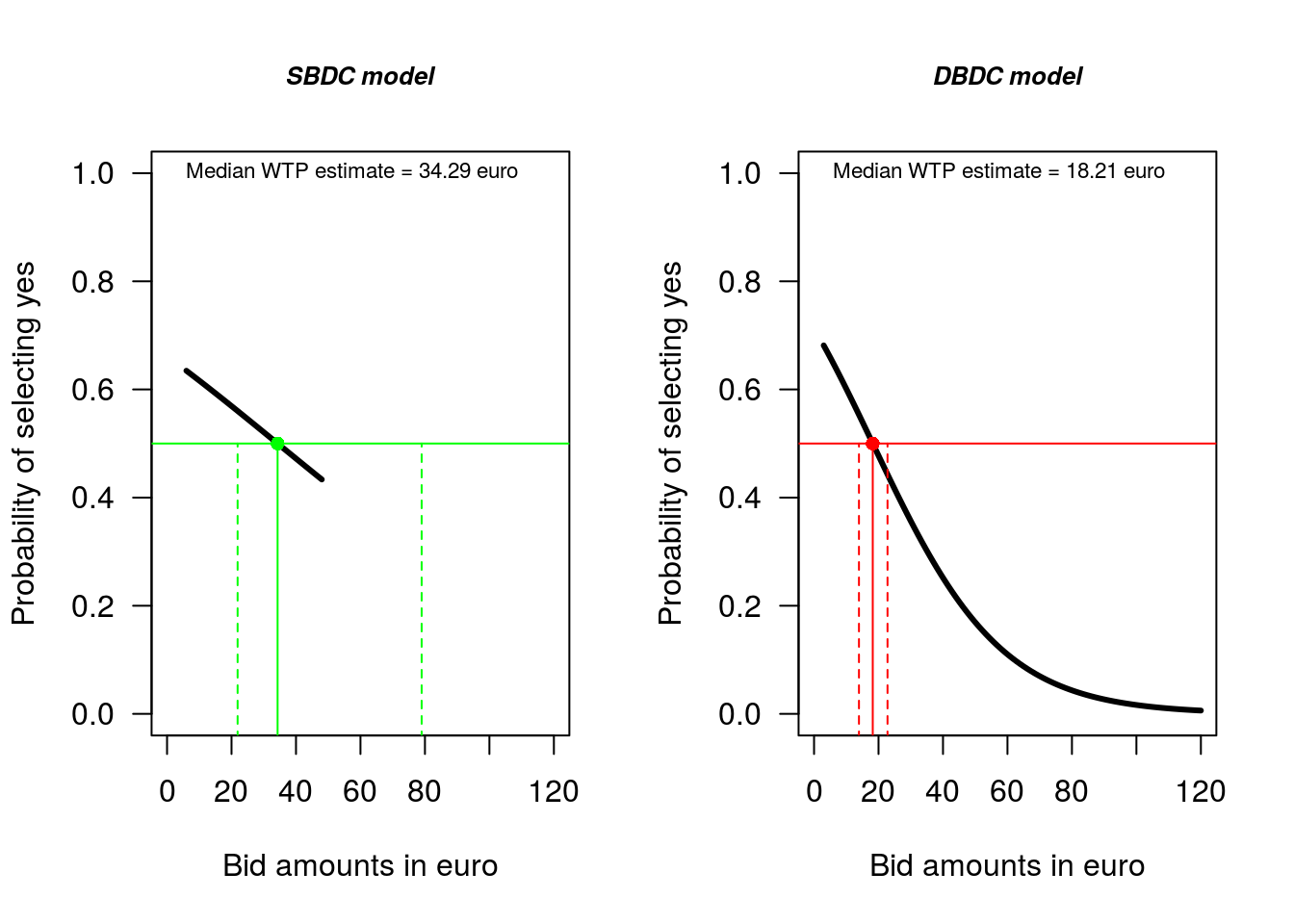

Figure 1.4: Comparison of simple and full model WTP estimates

In Figure 1.4, the solid black line is the estimate of the proportion of people that would say ‘yes’ (y-axis) to the various bid values (x-axis). The line is plotted only across the range of bid prices where we have data. So, in the case of the SBDC model this range is €6 to €48; and in the case of the DBDC model this range is €3 to €120.

Note the shape of the curve. The maximum and minimum proportion of people that can say ‘yes’ to a bid amount are ‘1’ and ‘0’. The model we fit ensures the predicted proportion falls within the zero one bound by fitting a non-linear model. This effect can not really be seen in the SBDC result, but can be clearly seen in the DBDC results.

The x-axis scale in both plots is the same. In each plot the solid horizontal line plots the median WTP estimate, and the dashed lines plot the 95% CI. The plot makes clear the dramatic improvement avaiable from asking a follow up question.

1.6 Extentions to look at individuals

The overall WTP infomation is generally what we focus on, and if the survey is based on a representative sample of the community, then this is a good meaure of community willingness to pay. However, sometimes we are interested in the WTP of specific groups. For example, we might be interested in the difference between the WTP of males and females. Or we might not have been able to get a representative sample, so we want to evaluate the WTP at some specific reference value.

Here we demonstate the process of evaluating WTP for different sub-groups and compare the WTP of young males and young females, with relatively high income. Recall that both income and age have been coded such that higher numbers are assocaited with older and richer people.

The extentions we need for the bootCI() function are minor. We just use the individual = data.frame(...) setting to specify the extra details. For the factor variable sex we specifiy the ‘level’. And for the other variables we just specify the numerical value.

The default setting for the simulations is to run the resampling ‘1,000’ times. This might take a while to run. As such, for illustation purposes, in the examples below we have also set the number of samples to draw as 100. For any actual research project it would be appropriate to just keep the default nboot setting.

The approach works in the same way whether you have a SBDC model or a DBDC model. Here we use the DBDC model results to illustate.

For young (age = 1) females (sex = "female") with a relatively high income (income = 5) we find WTP as:

set.seed(123)
bootCI(db.full, nboot = 100, individual = data.frame(sex = "female", age = 1, income = 5))

## the bootstrap confidence intervals
##                         Estimate     LB     UB
## Mean                      43.707 34.558 51.686
## truncated Mean            43.319 34.245 51.287
## adjusted truncated Mean   44.166 34.750 52.422
## Median                    41.322 29.989 50.586

So, for young females with a relatively high income the median WTP is €41.32 (95% CI:€29.99–€50.59)

For young (age = 1) males (sex = "male") with a relatively high income (income = 5) we find WTP as:

set.seed(123)
bootCI(db.full, nboot = 100, individual = data.frame(sex = "male", age = 1, income = 5))

## the bootstrap confidence intervals
##                         Estimate     LB     UB
## Mean                      48.313 38.383 59.902
## truncated Mean            47.814 37.993 58.808
## adjusted truncated Mean   49.022 38.692 61.720
## Median                    46.443 35.616 58.650

So, for young males with a relatively high income the median WTP is €46.44 (95% CI:€35.62–€58.65).

If we want to plot the different WTP curves for males and females, where we evaluate the other valuables at their mean values, then we: (i) set these values at their mean values and (ii) specify the range of values for the bid value (Figure 1.5):

F.WTP <- predict(db.full, type = "probability", newdata = data.frame(sex = "female", 
    age = mean(NP$age), income = mean(NP$income), bid1 = seq(from = 3, to = 120, 
        by = 1)))

M.WTP <- predict(db.full, type = "probability", newdata = data.frame(sex = "male", 
    age = mean(NP$age), income = mean(NP$income), bid1 = seq(from = 3, to = 120, 
        by = 1)))

plot(NULL, las = 1, xlab = "Bid amounts in euro", main = "Female", cex.main = 0.8, 
    font.main = 4, xlim = c(0, 120), ylab = "Proportion  of selecting yes", 
    ylim = c(0, 1), type = "l")
lines(3:120, F.WTP, lty = 1, lwd = 1)
abline(h = 0.5, lty = 1, col = "grey")
segments(x0 = 15.94, y0 = -1, x1 = 15.94, y1 = 0.5, col = "black", lty = 2)

plot(NULL, las = 1, xlab = "Bid amounts in euro", main = "Male", cex.main = 0.8, 
    font.main = 4, xlim = c(0, 120), ylab = "Proportion  of selecting yes", 
    ylim = c(0, 1), type = "l")
lines(3:120, M.WTP, lty = 1, lwd = 1)
abline(h = 0.5, lty = 1, col = "grey")
segments(x0 = 21.06, y0 = -1, x1 = 21.06, y1 = 0.5, col = "black", lty = 3)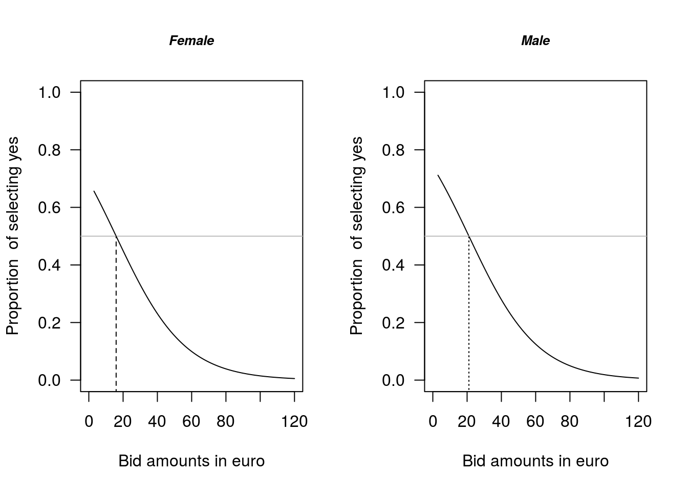

Figure 1.5: Comparison of female and male WTP estimates

1.7 An overview of a contingent valuation research report

So far this guide has covered how to estimate WTP from a CV study. In practice, the results from a study will need to be written up and presented to a target audience. A common format for writting up research report results is the: Introduction, Methods, Results, Discussion (IMRD) format. Below, the content of each section of a CV report that follows the IMRD format is described.

1.7.1 Introduction

Here the points to cover will include:

• An overview of the research question and why it is important
• Some relevant background information that places the current survey in context
• Some material that describes why it is neccessary to undertake a primary CV study
• Some key relevant literature to set up the current state of knowledge. For example, how much is known about WTP estimates for similar situations in other countries, or WTP for other things in the sample jurisdiction?

1.7.2 Methods

Here the points to cover will include:

• An explicit statement of the survey question, and the pattern of bid information for the first question and the follow up question: A table is one way to display this information (Table 1.1).
• Explicit details of the way the data was collected, and information on any workshops that may have been held with local community groups to refine the questions.
• Details on the data set and information that compares the survey sample data set with national (or local) population parameters for key variables such as: age, income, gender proportion, eductaion level, etc. It is important to know whether or not the sample data is representative or not.
• Details of the method of estimation used: which is likely to be a DBDC CV survey using the DCchoice package for R.
• Details of the model selection process; the variables considered; the model selection criteria, e.g. minimise AIC or BIC; individual variable statistical significance, based on theory and other literature; etc.

Table 1.1: Example bid table

Bid amount	a	b	c	d
Initial question bid	6	12	24	48
Follow up question low	3	6	12	24
Follow up question higt	12	24	48	120

1.7.3 Results

In the results section there will be two main areas of focus. Reporting details for the core model, and reporting median WTP information. Generally, this information will be reported in table format. For completness, you may also want to report results for comparison models, and mean WTP information. Some indicative examples of tables that might feature in the Results section are below (Tables 1.2 and 1.3). You may also want to include some plots to demostrate the way that WTP varies with, say gender.

Table 1.2: Example regression results table

Variable	Est.	\(p\) value	Est.	\(p\) value
Intercept	\(0.835\)	\(2.2 \times 10^{-16}\)	\(1.422\)	\(0.0003\)
Bid	\(-0.046\)	\(2.2 \times 10^{-16}\)	\(-0.050\)	\(2.2 \times 10^{-16}\)
Age	-	-	\(-0.325\)	\(1.7 \times 10^{-5}\)
Female	-	-	\(-0.256\)	\(0.2364\)
Income	-	-	\(0.245\)	\(0.0056\)
Log-likelihood value	\(-406.02\)	-	\(-386.64\)	-
AIC	\(816.04\)	-	\(783.29\)	-

Table 1.3: Example WTP (euros) and 95%CI table

Group	Median	Lower bound	Upper bound
Overall	18.20	13.93	22.79
Males	21.06	16.82	28.06
Females	15.94	10.94	20.82

Note that we find the male and female WTP values, and 95% CI using:

bootCI(db.full, nboot = 100, individual = data.frame(sex = "male", age = mean(NP$age), 
    income = mean(NP$income)))

bootCI(db.full, nboot = 100, individual = data.frame(sex = "female", age = mean(NP$age), 
    income = mean(NP$income)))

In terms of relevant plots, the overall WTP distribution, and the distribution of WTP across, say males and females, is likely to be valuable (Figure 1.6). You can also add confidence interval information for the median estimate as additional lines to the plot, if desired.

plot(db.full, las = 1, xlab = "Bid amounts in euro", main = "Overall results", 
    cex.main = 0.8, font.main = 4, xlim = c(0, 120), ylab = "Proportion of selecting yes", 
    ylim = c(0, 1), lwd = 2)
abline(h = 0.5, lty = 3, col = "grey", lwd = 1)
segments(x0 = 18.2, y0 = -1, x1 = 18.2, y1 = 0.5, col = "black", lty = 1, lwd = 2)
legend("topright", legend = c("Overall WTP"), lty = 1, lwd = 1, bty = "n", col = "black", 
    cex = 0.7)

plot(NULL, las = 1, xlab = "Bid amounts in euro", main = "Gender specific results", 
    cex.main = 0.8, font.main = 4, xlim = c(0, 120), ylab = "Proportion of selecting yes", 
    ylim = c(0, 1))
lines(3:120, F.WTP, lty = 2, lwd = 2)
lines(3:120, M.WTP, lty = 4, lwd = 2)
abline(h = 0.5, lty = 3, col = "grey")
segments(x0 = 15.94, y0 = -1, x1 = 15.94, y1 = 0.5, col = "black", lty = 2, 
    lwd = 2)
segments(x0 = 21.06, y0 = -1, x1 = 21.06, y1 = 0.5, col = "black", lty = 4, 
    lwd = 2)
legend("topright", legend = c("Female WTP", "Male WTP"), lty = c(2, 4), lwd = c(1, 
    1), bty = "n", col = c("black", "black"), cex = 0.7)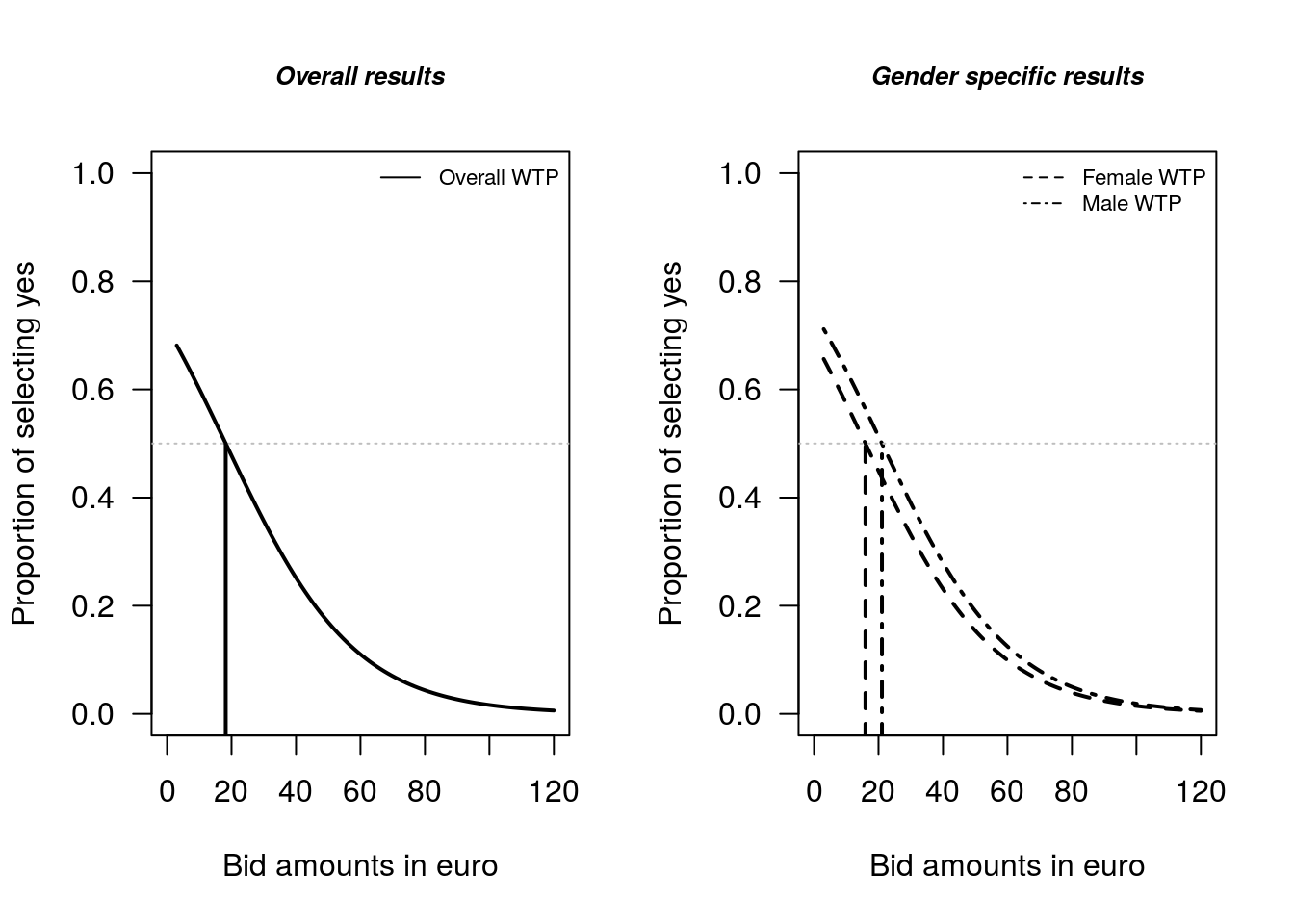

Figure 1.6: Comparison of Female and Male WTP estimates

1.7.4 Discussion

Here is where you translate the WTP information to the relevant context. For example, if the issue was local air polution in an area you could calculate the total WTP of the relevant region and compare this value to the cost of pollution mitigation measures. If the issue is conservation, the total value estimate could be compared to the cost of the relevant environmental program. In many cases the discussion section may include a formal cost-benefit assessment.

Regardless of the specific approach taken to set out the discussion it is important that the policy implications of the WTP estimate information are set out in the discussion.

References

Aizaki, H., T. Nakatani, and K. Sato. 2014. Stated Preference Methods Using R. Florida, USA: CRC Press. https://doi.org/10.1201/b17292.

Bateman, I. J., R. T. Carson, B. Day, M. Hanemann, N. Hanley, T. Hett, M. Jones-Lee, et al., eds. 2002. Economic Valuation with Stated Preference Techniques: A Manual. Cheltenham, UK: Edward Elgar.

Bateman, I. J., and K. G. Willis, eds. 1999. Valuing Environmental Preferences: Theory and Practice of the Contingent Valuation Methods in the US, EU, and Developing Countires. New York: Oxford University Press.

Carson, R. T., and W. M. Hanemann. 2005. “Contingent Valuation.” In Handbook of Environmental Economics, Volume 2, edited by K. G. Mäler and J. R. Vincent, 821–936. New York: Elsevier.

Croissant, Y., and S. Graves. 2020. Ecdat: Data Sets for Econometrics. https://CRAN.R-project.org/package=Ecdat.

Efron, B., and R. Tibshirani. 1993. An Introduction to the Bootstrap. New York: Chapman & Hall.

Hole, A. R. 2007. “A Comparison of Approaches to Estimating Confidence Intervals for Willingness to Pay Measures.” Health Economics 16: 827–40. https://doi.org/10.1002/hec.1197.

Krinsky, I., and A. L. Robb. 1986. “On Approximating the Statistical Properties of Elasticities.” The Review of Economics and Statistics 68: 715–19. https://doi.org/10.2307/1924536.

Krinsky, I., and A. L. Robb. 1986. “On Approximating the Statistical Properties of Elasticities.” The Review of Economics and Statistics 68: 715–19. https://doi.org/10.2307/1924536.

1990. “On Approximating the Statistical Properties of Elasticities: A Correction.” The Review of Economics and Statistics 72: 189–90. https://doi.org/10.2307/2109761.

Nakatani, T., H. Aizaki, and K. Sato. 2020. DCchoice: An R Package for Analyzing Dichotomous Choice Contingent Valuation Data. https://CRAN.R-project.org/package=DCchoice.

R Core Team. 2021a. An Introduction to R. https://CRAN.R-project.org/manuals.html.

R Core Team. 2021b. R: A Language and Environment for Statistical Computing. Vienna, Austria: R Foundation for Statistical Computing. https://www.R-project.org/.

RStudio. 2020. RStudio Desktop. https://www.rstudio.com/.

Zeileis, A., and T. Hothorn. 2002. “Diagnostic Checking in Regression Relationships.” R News 2 (3): 7–10. https://CRAN.R-project.org/doc/Rnews/.