Chapter 3 An Illustrative Example of Case 1 Best–Worst Scaling
Authors: Hideo Aizaki and James Fogarty
Latest Revision: 9 March 2021 (First Release: 30 March 2018)
3.1 Before you get started
This tutorial, which is a revised version of the manual for the package support.BWS, presents the entire process of Case 1 (object case) best–worst scaling (BWS)—from constructing the choice sets to analyzing responses using R (R Core Team 2021b). The demonstration assumes some familiarity with R. If you are completely unfamiliar with R, you are advised to consult R Core Team (2021a) and the other support materials before attempting the material below.
NOTE: this tutorial is based on the support.BWS package version 0.4-3 or later.
3.2 Overview
After outlining the three variants of BWS, this section briefly explains Case 1 BWS. For details, please refer to previous works such as Louviere, Flynn, and Marley (2015).
3.2.1 Three variants of BWS
BWS is a method for measuring individuals’ preferences for items (objects or levels). BWS constructs choice sets by forming various item combinations and then asks respondents to select the best and worst items from each choice set. According to the format of the choice sets, BWS is divided into three variants: Case 1, Case 2, and Case 3. Case 1 BWS—or maximum difference scaling (MaxDiff) (Finn and Louviere 1992)—lists the items (objects) evaluated by respondents; and constructs a number of different subsets of the items from the list using the experimental design. Each of the subsets is presented as a choice set to respondents, who are then asked to select the best (or most important) and worst (or least important) items in the choice set. This question is repeated until all the subsets are evaluated. In constrast, Case 2 and 3 BWS list attributes and their levels. Case 2 (profile case) BWS constructs various combinations of attribute levels (i.e., profiles) and then ask respondents to select the best and worst levels in each profile. Case 3 (multi-profile) BWS asks respondents to select the best and worst profiles in each choice set including three or more profiles. Alternatives in a Case 2 BWS question correspond to levels presented in a choice set, whereas those in a Case 3 BWS question correspond to profiles presented in a choice set.
As an example, to highlight the differences in the choice set formats of the three variants of BWS, we consider consumers’ valuations of apples:
- A Case 1 BWS study may focus on seven attributes of apples such as country-of-origin, cultivation method, variety, appearance, size, traceability, and price, and ask respondents to select the most and least important of four attributes in each question (Figure 3.1).
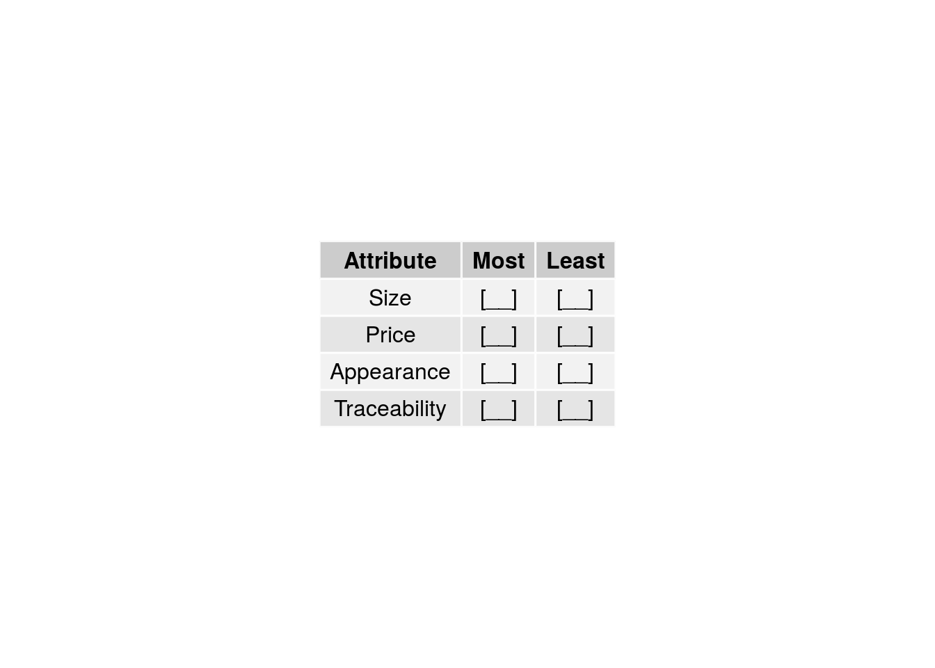
Figure 3.1: Example Case 1 BWS question.
- A Case 2 BWS study may focus on four attributes such as country of origin, cultivation method, traceability, and price, define two or more levels for each attribute, and ask respondents to select the most and least preferred of the levels shown in each question (Figure 3.2).
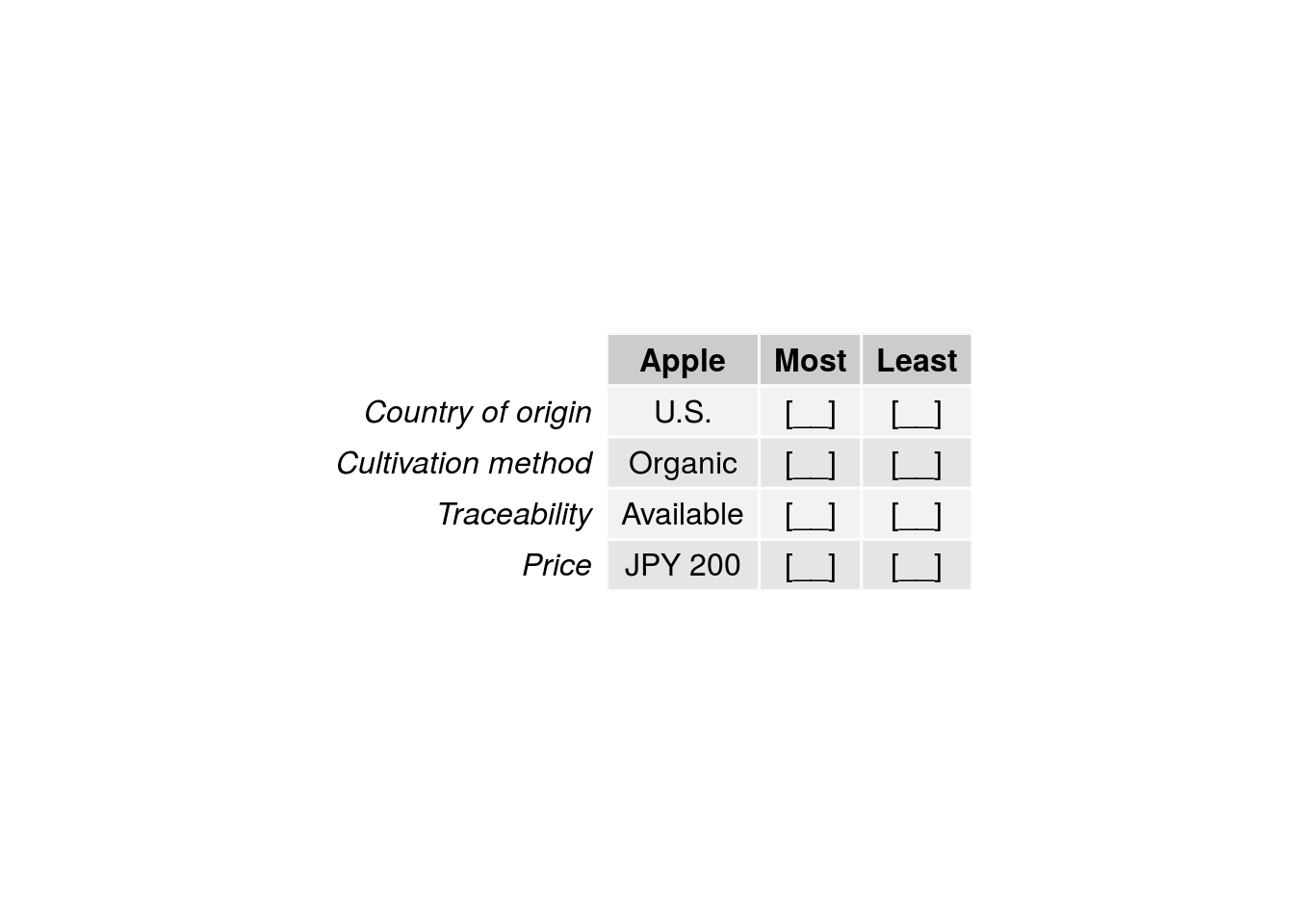
Figure 3.2: Example Case 2 BWS question.
- A Case 3 BWS study may focus on four attributes such as country of origin, cultivation method, traceability, and price, define two or more levels for each attribute, and ask respondents to select the most and least preferred apples in each question (Figure 3.3).
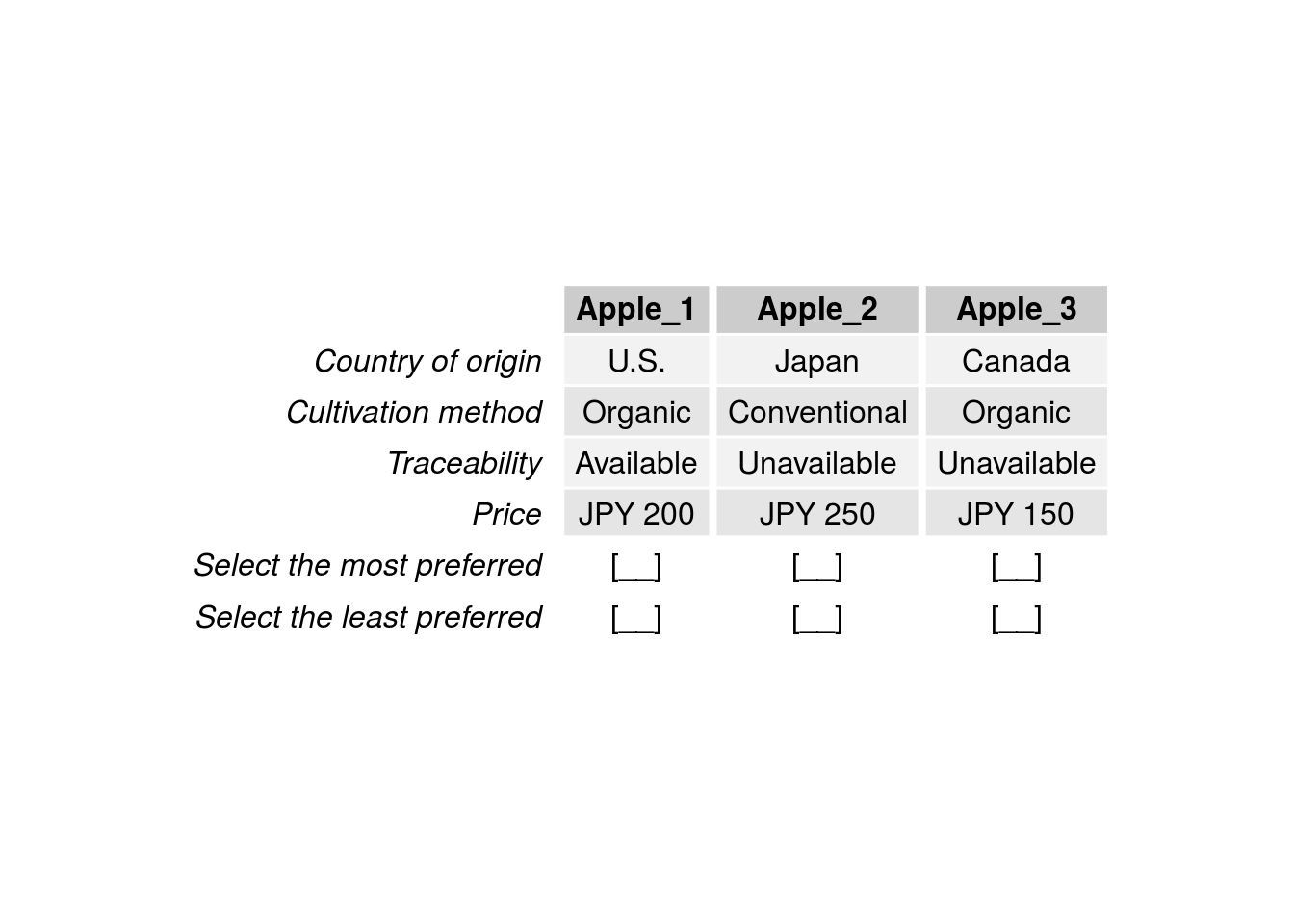
Figure 3.3: Example Case 3 BWS question.
3.2.2 Case 1 BWS
Many Case 1 BWS studies used a balanced incomplete block design (BIBD) to construct choice sets (e.g., Auger et al., 2007). BIBD is a category of designs in which a subset of treatments is assigned to each block. The features of a BIBD are expressed by the number of treatments (items), size of a block (number of items per question), number of blocks (questions), number of replications of each treatment (item), and frequency that each pair of treatments (items) appears in the same block (question). Each row corresponds to a question; the number of columns is equal to the number of items per question; and the level values correspond to item identification numbers. For example, in a study with seven items, ITEM1, ITEM2, …, and ITEM7, and a BIBD with seven rows, four columns, and seven level values (1, 2, …, 7), if a row in the BIBD contains values of 1, 4, 6, and 7, a set containing ITEM1, ITEM4, ITEM6, and ITEM7 is presented in a question, corresponding to the row.
There are two approaches for analyzing responses to Case 1 BWS questions: the counting approach and the modeling approach. The counting approach calculates several types of scores on the basis of the number of times (i.e., the frequency or count) item \(i\) is selected as the best (\(B_{in}\)) or worst (\(W_{in}\)) item among all the questions for respondent \(n\). These scores are roughly divided into two categories: disaggregated (individual-level) scores and aggregated (total-level) scores (Finn and Louviere 1992; Lee, Soutar, and Louviere 2007a; Cohen 2009; Mueller, Francis, and Lockshin 2009).
- The first category includes a disaggregated BW score and its standardized score:
\[\begin{equation} BW_{in} = B_{in} - W_{in}, \end{equation}\]
\[\begin{equation} std.BW_{in} = \frac{BW_{in}}{r}, \end{equation}\]
where \(r\) is the frequency with which item \(i\) appears across all questions.
- The frequency with which item \(i\) is selected as the best item across all questions for \(N\) respondents is defined as \(B_{i}\). Similarly, the frequency with which item \(i\) is selected as the worst item is defined as \(W_{i}\) (i.e., \(B_{i} = \sum_{n=1}^{N} B_{in}\), \(W_{i} = \sum_{n=1}^{N} W_{in}\)). The second category includes the aggregated versions of \(BW_{in}\) and \(std.BW_{in}\), as well as the square root of the ratio of \(B_{i}\) to \(W_{i}\) and its standardized score:
\[\begin{equation} BW_{i} = B_{i} - W_{i}, \end{equation}\]
\[\begin{equation} std.BW_{i} = \frac{BW_{i}}{Nr}, \end{equation}\]
\[\begin{equation} sqrt.BW_{i} = \sqrt{\frac{B_{i}}{W_{i}}}, \end{equation}\]
\[\begin{equation} std.sqrt.BW_{i} = \frac{sqrt.BW_{i}}{max.sqrt.BW}, \end{equation}\]
where \(max.sqrt.BW\) is the maximum value of \(sqrt.BW_{i}\).
The modeling approach uses discrete choice models to analyze responses. When using the modeling approach, you must select a model type according to your assumptions on the respondents’ responses to the Case 1 BWS questions. Then, a dataset must be formatted as per the selected model. There are three standard models: maxdiff (paired), marginal, and marginal sequential (Flynn et al. 2007, 2008; Hensher, Rose, and Greene 2015; Louviere, Flynn, and Marley 2015). Although the three models commonly assume that the respondents derive utility for each item in a choice set, the assumption of how they select the best and worst items from the set differs among the three models. The following text explains the three models on the basis of common assumptions that \(m\) items exist in a choice set (a question) and that respondents select item \(i\) as the best item and item \(j\) (\(i \neq j\)) as the worst item.
The maxdiff model assumes that respondents make their selections because the difference in utility between \(i\) and \(j\) represents the greatest utility difference among \(m \times (m - 1)\) possible utility differences, where \(m \times (m - 1)\) is the number of possible pairs in which item \(i\) is selected as the best item and item \(j\) is selected as the worst item from \(m\) items.
The marginal model assumes that respondents select item \(i\) as the best item from \(m\) possible best items in the choice set, and select item \(j\) as the worst item from \(m\) possible worst items. Therefore, the model assumes that the utilities for items \(i\) and \(j\) are the maximum and minimum, respectively, among the utilities of all \(m\) items.
The marginal sequential model assumes that respondents sequentially select item \(i\) as the best item from \(m\) items in the choice set and then select item \(j\) as the worst item from the remaining \(m - 1\) items.
The probability of selecting item \(i\) as the best item and item \(j\) as the worst item from a choice set \(C\) for each model can be expressed using the conditional logit model with the systematic component of utility \(v\), as follows.
- The maxdiff model:
\[\begin{equation} \mathrm{Pr}(\mathrm{best} = i, \mathrm{worst} = j) = \frac{\exp{(v_{i} - v_{j})}}{\sum_{p, q \subset C, p \neq q} \exp{(v_{p} - v_{q})}}. \end{equation}\]
- The marginal model:
\[\begin{equation} \mathrm{Pr}(\mathrm{best} = i, \mathrm{worst} = j) = \frac{\exp{(v_{i})}}{\sum_{p \subset C} \exp{(v_{p})}}\frac{\exp{(-v_{j})}}{\sum_{p \subset C} \exp{(-v_{p})}}. \end{equation}\]
- The marginal sequential model:
\[\begin{equation} \mathrm{Pr}(\mathrm{best} = i, \mathrm{worst} = j) = \frac{\exp{(v_{i})}}{\sum_{p \subset C} \exp{(v_{p})}}\frac{\exp{(-v_{j})}}{\sum_{q \subset C - i} \exp{(-v_{q})}}. \end{equation}\]
The share of preference for item \(i\) (\(\mathit{SP}_{i}\)) measures the extent of the relative importance between items (Cohen 2003; Cohen and Neira 2004; Lusk and Briggeman 2009): \[\begin{equation} \mathit{SP}_{i} = \frac{\exp(v_{i})}{\sum_{t=1}^{T}\exp(v_{t})}. \end{equation}\]
3.3 Packages for Case 1 BWS
We use four CRAN packages—support.BWS (Aizaki 2021), crossdes (Sailer 2013), dfidx (Croissant 2020a), and mlogit (Croissant 2020b)—to explain how to implement Case 1 BWS in R. The support.BWS package provides functions that convert a BIBD into Case 1 BWS questions, create a dataset for analysis from the BIBD and the responses to the questions, and calculate BWS scores. The find.BIB() function in the crossdes package can construct BIBDs, whereas the mlogit() function in the mlogit package is used to fit the conditional logit model and the random parameters logit model. The mlogit() function is also appropriate for the other advanced discrete choice models (see vignettes in mlogit for details). The mlogit() function needs a dataset in a special format, the S3 class "dfidx". We can convert the dataset created using support.BWS into that of the S3 class "dfidx" with the dfidx() function in dfidx.
Assuming that the packages have been installed, first we load the packages needed for the example into the current R session:
Note that we printed out four digits in the example. To set the same appearance format in R, execute
3.4 Designing a choice situation
We will explain how to use the R functions on the basis of an actual survey regarding Japanese consumer preferences for rice characteristics. Respondents were asked to select the most and least important rice characteristics when purchasing.
For the first step of implementing Case 1 BWS, we assume that rice consists of the following seven characteristics (variable names are in parenthesis):
- Place of origin (
origin), - Variety (
variety), - Price (
price), - Taste (
taste), - Safety (
safety), - Wash-free rice (
washfree), - Milling date (
milling),
where wash-free rice means that consumers do not need to wash the rice with water before cooking it.
3.5 Generating a BIBD
The second step is the preparation of a BIBD corresponding to the designed choice situation. The find.BIB() function is available for creating BIBDs. For the survey, we created a BIBD with seven treatments (items), seven rows (questions), and four columns (items per question) using the find.BIB() function:
set.seed(8041) # a random seed value can be anything
des <- find.BIB(
  trt = 7, # seven treatments
  b   = 7, # seven rows
  k   = 4) # four columns
des
## [,1] [,2] [,3] [,4]
## [1,] 2 3 4 7
## [2,] 1 2 3 6
## [3,] 1 2 5 7
## [4,] 2 4 5 6
## [5,] 1 3 4 5
## [6,] 3 5 6 7
## [7,] 1 4 6 7We can see that the resultant BIBD consists of seven integer values from 1 to 7 because we have set seven treatments: these values correspond to item numbers defined in the next step. The find.BIB() function searches for a BIBD using random numbers. This means that the resultant BIBDs vary when implementing the find.BIB() function. As such, the seed for the random number generator can be set to any value (i.e., 8041 in this example) in order to reproduce the same BIBD in the future. Furthermore, we have to use the isGYD() function in the crossdes package to check whether the resultant design is a BIBD:
##
## [1] The design is a balanced incomplete block design w.r.t. rows.
The result above indicates that the resultant design is a BIBD.
NOTE: Case 1 BWS studies have used various BIBDs. Below is the limited list of example BIBD configurations: \(trt = 6\), \(b = 10\), and \(k = 3\) (e.g., Hein et al. 2008; Hoek et al. 2011); \(trt = 7\), \(b = 7\), and \(k = 3\) (e.g., Jaeger and Cardello 2009; Loureiro and Arcos 2012); \(trt = 9\), \(b = 12\), and \(k = 6\) (e.g., Dumbrell, Kragt, and Gibson 2016; Lee, Soutar, and Louviere 2007b); \(trt = 11\), \(b = 11\), and \(k = 5\) (e.g., Mazanov, Huybers, and Connor 2012; Gallego et al. 2012); and \(trt = 13\), \(b = 13\), and \(k = 4\) (e.g., Jaeger, Danaher, and Brodie 2009; Wang et al. 2011). Catalogs of BIBDs are available in books on experimental design such as Cochran and Cox (1957).
3.6 Creating questions
The third step is the creation of Case 1 BWS questions. The bws.questionnaire() function converts a BIBD into a series of Case 1 BWS questions, and then displays the resultant questions on an R console. In preparation, the names of the items are stored in the vector items.rice:
Note that the order of the items in the vector corresponds to the item numbers, i.e., the order of level values used in the BIBD created above. This means that the item numbers of origin, variety, price, taste, safety, washfree, and milling are 1, 2, 3, 4, 5, 6, and 7, respectively.
Then, we obtain a series of Case 1 BWS questions from the BIBD using the bws.questionnaire() function:
bws.questionnaire(choice.set = des, # dataframe or matrix containing a BIBD
                  design.type = 2,  # 2 if a BIBD is assgined to choice.set
                  item.names = items.rice) # names of items shown in questions
Q1
 Best Items   Worst
 [ ]  variety [ ]
 [ ]  price   [ ]
 [ ]  taste   [ ]
 [ ]  milling [ ]

 ...

Q7
 Best Items    Worst
 [ ]  origin   [ ]
 [ ]  taste    [ ]
 [ ]  washfree [ ]
 [ ]  milling  [ ]
The first row of the BIBD created above consists of four values, such as 2, 3, 4, and 7; thus, the first question (Q1) consists of four characteristics, such as variety, price, taste, and milling date, respectively. The last row of the BIBD consists of 1, 4, 6, and 7; thus, the last question (Q7) consists of place of origin, taste, wash-free rice, and milling date, respectively.
3.7 Conducting a survey
The fourth step entails conducting a questionnaire survey using the Case 1 BWS questions created above. We will use the results of previously conducted survey in lieu of this step.
3.8 Creating a dataset
3.8.1 Preparing a dataset including responses to the questions
The fifth step is the creation of a dataset for analysis by combining the BIBD generated in the second step with the responses to the Case 1 BWS questions gathered in the fourth step. In this example, the responses are stored in the dataset ricebws1 in the support.BWS package. This is loaded into the current session as follows:
## [1] 90 18## [1] "id" "b1" "w1" "b2" "w2" "b3" "w3" "b4" "w4" "b5"
## [11] "w5" "b6" "w6" "b7" "w7" "age" "hp" "chem"As shown above, the dataset contains 90 observations (respondents) with the following 18 variables:
id: The respondents’ identification number (id).b1–w7: Values corresponding to the responses to the Case 1 BWS questions;bdenotes a response as the best item,wdenotes a response as the worst item, and the numbers1to7correspond to the BWS question numbers.age: The respondents’ age category:1,2, and3represent under 40, 40–59, and over 60, respectively.hp: The highest price for 5 kg of rice that respondents have paid during last six months:1,2, and3represent to under 1,600 JPY, 1,600–2,100 JPY, and over 2,100 JPY, respectively.chem: The respondents’ subjective value of rice grown with low-agrochemicals, taking the value of1if respondents recognize the value of low-agrochemical rice or0otherwise.
After conducting a survey, you will have to create a respondent dataset based on the completed questionnaires. The structure of the respondent dataset must follow that of ricebws1—it must include the respondents’ id variable and the response variables, each indicating which items are selected as the best and worst items for each question. The response variables must be named using two different letters (words) corresponding to the best and worst selections and integer values distinguishing BW questions. This is because a function for creating a dataset for BWS1 analysis (i.e., bws.dataset()), which will be explained later, uses the function reshape() internally to change the dataset from wide to long format. The response variables must also be arranged in the respondent dataset such that the best items alternate with the worst, by question. For example, if the letter b is used to create the response variables for the best selections; the letter w is used to create the response variables for the worst selections; and there are seven BWS questions, the variables are b1 w1 b2 w2 … b7 w7. Here, bi and wi are respectively the selections for the best and worst items in the i-th question. The row numbers of the items or the item numbers selected as the best and worst items are stored in the response variables. For example, suppose a respondent was asked to answer Q1 mentioned above, and they selected variety and milling date as the best and worst characteristics, respectively. In the row number format, the response variables b1 and w1, corresponding to the respondent’s answer to this question, take values of 1 (= the items in the first row) and 4 (= the attribute-level in the fourth row). In the item number format, the response variables b1 and w1 take values of 2 (= the item number of variety) and 7 (= the item number of milling date). The name of the id variable is left to the discretion of the user. Variables regarding respondents’ characteristics are included in your respondent dataset if necessary.
3.8.2 Combining the design and the responses
After preparing the respondent dataset, a dataset is created for analysis using the bws.dataset() function (Step 6). In preparation for using this function, we store the names of the response variables used in the respondent dataset ricebws1 in the vector response.vars:
## [1] "b1" "w1" "b2" "w2" "b3" "w3" "b4" "w4" "b5" "w5" "b6" "w6" "b7" "w7"Although the datasets for the maxdiff, marginal, and marginal sequential models can be created using the bws.dataset() function, this example assumes that the respondents answer the BWS questions on the basis of the maxdiff model (the code excerpts for creating the datasets for the marginal model and the marginal sequential model are shown in Appendix 3A):
# Dataset for the maxdiff model
md.data <- bws.dataset(
  data = ricebws1, # data frame containing response dataset
  response.type = 1, # format of response variables: 1 = row number format
  choice.sets = des, # choice sets
  design.type = 2, # 2 if a BIBD is assgined to choice.sets
  item.names = items.rice, # the names of items
  id = "id", # the name of respondent id variable
  response = response.vars, # the names of response variables
  model = "maxdiff") # the type of dataset created by the function is the maxdiff model
dim(md.data)
## [1] 7560 19The data frame md.data consists of 7,560 rows (= 90 respondents \(\times\) 7 BWS questions \(\times\) 12 possible pairs per BWS question [ = \(4 \times 3\)]) and 19 columns (variables).
The following output displays the 19 variables in the md.data corresponding to the 12 possible response pairs (PAIR = 1 to 12) in the first question (Q = 1) for respondent 1 (id = 1). The variables BEST and WORST show the item numbers of the best and worst items in a possible pair—e.g., the first row in the following output indicates a possible pair in which variety (item number = 2) is treated as the best characteristic and price (item number = 3) is treated as the worst characteristic. The item variables from columns origin to milling are created as dummy variables with reversed sign when the items are treated as the possible worst. Therefore, the first row indicates that the values of the item variables variety and price are 1 and -1, respectively, and the value of the remaining item variables are 0. These item variables are used as independent variables in the modeling approach. The variable RES is a response variable used as a dependent variable in the modeling approach, taking a value of TRUE if a possible pair is actually selected by the respondent, and FALSE otherwise. In this example, the value of RES is TRUE in the 10th row, and FALSE in the remaining 11 rows. This means that respondent 1 selected milling date and variety as the best and worst characteristics. Note that the structure of the resultant dataset differs with the model variants (See Appendix 3A for the structures of the other models).
##    id Q PAIR BEST WORST RES.B RES.W   RES origin variety price taste safety
## 1   1 1    1    2     3     7     2 FALSE      0       1    -1     0      0
## 2   1 1    2    2     4     7     2 FALSE      0       1     0    -1      0
## 3   1 1    3    2     7     7     2 FALSE      0       1     0     0      0
## 4   1 1    4    3     2     7     2 FALSE      0      -1     1     0      0
## 5   1 1    5    3     4     7     2 FALSE      0       0     1    -1      0
## 6   1 1    6    3     7     7     2 FALSE      0       0     1     0      0
## 7   1 1    7    4     2     7     2 FALSE      0      -1     0     1      0
## 8   1 1    8    4     3     7     2 FALSE      0       0    -1     1      0
## 9   1 1    9    4     7     7     2 FALSE      0       0     0     1      0
## 10  1 1   10    7     2     7     2  TRUE      0      -1     0     0      0
## 11  1 1   11    7     3     7     2 FALSE      0       0    -1     0      0
## 12  1 1   12    7     4     7     2 FALSE      0       0     0    -1      0
##    washfree milling STR age hp chem
## 1         0       0 101   3  2    1
## 2         0       0 101   3  2    1
## 3         0      -1 101   3  2    1
## 4         0       0 101   3  2    1
## 5         0       0 101   3  2    1
## 6         0      -1 101   3  2    1
## 7         0       0 101   3  2    1
## 8         0       0 101   3  2    1
## 9         0      -1 101   3  2    1
## 10        0       1 101   3  2    1
## 11        0       1 101   3  2    1
## 12        0       1 101   3  2    1
3.9 Measuring preferences
3.9.1 The counting approach
The final step is the measurement of preferences for the items by analyzing the responses with the counting or modeling approach. Even if you follow the modeling approach in your study, you should partly undertake the counting approach because looking at descriptive features of responses to BWS questions is also useful for the modeling approach.
The bws.count() function calculates the best (B), worst (W), best-minus-worst (BW), and standardized BW scores for each respondent. The function has two arguments: data and cl. A data frame containing the dataset generated from the bws.dataset() function is assigned to the argument data. When using this function with the argument cl = 1, it returns an object of the S3 class "bws.count" containing disaggregated scores and aggregated scores in list format. When using this function with the argument cl = 2, it returns an object of the S3 class "bws.count2", which inherits from the S3 class "data.frame", including disaggregated B, W, BW, and standardized BW scores, respondent id variable, and variables regarding respondent characteristics. Although the default is the argument cl = 1 for backward compatibility, the argument cl = 2 is recommended. Therefore, we calculate the BWS scores using bws.count() with the dataset for the maxdiff model and the argument cl = 2 (Note that the datasets for the marginal and marginal sequential models are also available to bws.count()):
## [1] 90 32## [1] "id" "b.origin" "b.variety" "b.price" "b.taste"
## [6] "b.safety" "b.washfree" "b.milling" "w.origin" "w.variety"
## [11] "w.price" "w.taste" "w.safety" "w.washfree" "w.milling"
## [16] "bw.origin" "bw.variety" "bw.price" "bw.taste" "bw.safety"
## [21] "bw.washfree" "bw.milling" "sbw.origin" "sbw.variety" "sbw.price"
## [26] "sbw.taste" "sbw.safety" "sbw.washfree" "sbw.milling" "age"
## [31] "hp" "chem"We can see that the object cs consists of 90 rows (respondents) and 32 columns (variables), containing id variable, B, W, BW, and standardized BW score variables, and three respondent characteristic variables (i.e., age, hp, and chem).
To understand the relative importance of items among individuals, we should note the means of the BWS scores of items as well as the variances (standard deviations). The graphical presentation of individual BWS scores allows us to easily read the relationship between the means and standard deviations of BWS scores. The plot() method for the S3 class "bws.count2" draws the relationship between the means and standard deviations of B, W, or BW scores (Figure 3.4):
plot(
  x = cs,
  score = "bw",       # BW scores are used
  pos = 4,            # Labels are added to the right of the points
  ylim = c(1.6, 2.3), # the y axis ranges from 1.6 to 2.3
  xlim =c(-3, 3))     # the x axis ranges from -3 to 3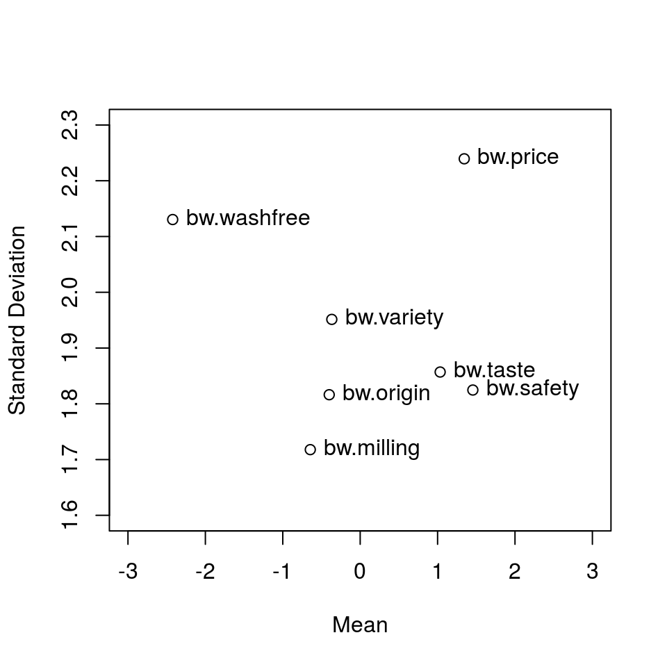
Figure 3.4: Graphical presentation of individual BW scores
Figure 3.4 reveals that the three rice characteristics of price, taste, and safety are similarly important, but the variance of price is larger than those of taste and safety. Therefore, the importance of price differs largely among individuals.
To investigate the heterogeneity in detail, we can draw bar plots of BWS scores using the barplot() method for the S3 class "bws.count2" (Figure 3.5):
par(mar = c(5, 4, 2, 1))
barplot(
  height = cs,
  score = "bw",    # BW scores are used
  mfrow = c(3, 3)) # Bar plots are drawn in a 3-by-3 array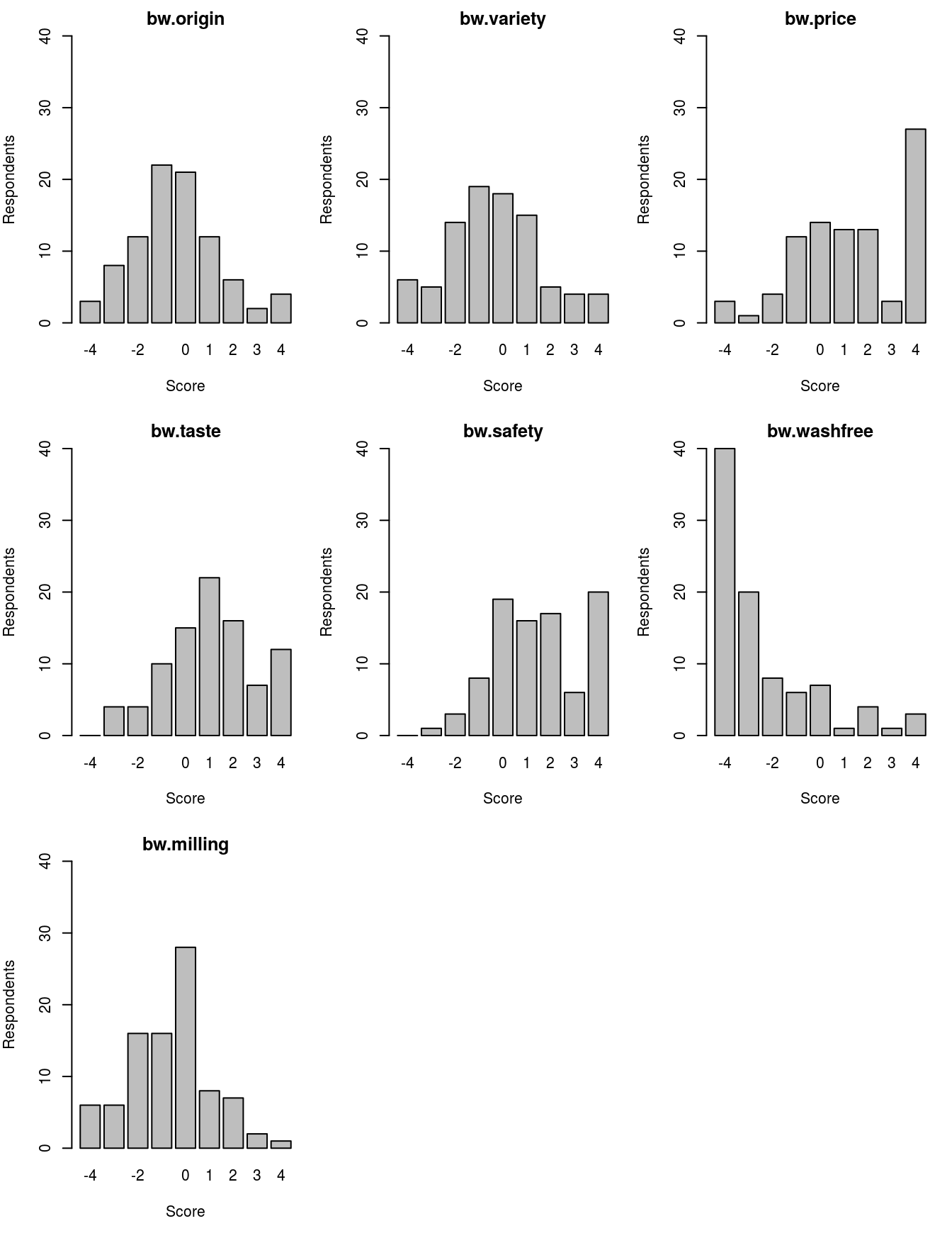
Figure 3.5: Bar plots of BW scores.
Figure 3.5 reveals us that respondents who have a BW score of 4 for price comprise a larger group, resulting in the large variance of the BW score for rice.
The barplot() method for the S3 class "bws.count2" can be also used to draw mean BWS scores (Figure 3.6):
par(mar = c(5, 7, 1, 1))
barplot(
  height = cs,
  score = "sbw", # Standardized BW scores are used
  mean = TRUE,   # Bar plot of mean scores is drawn
  las = 1)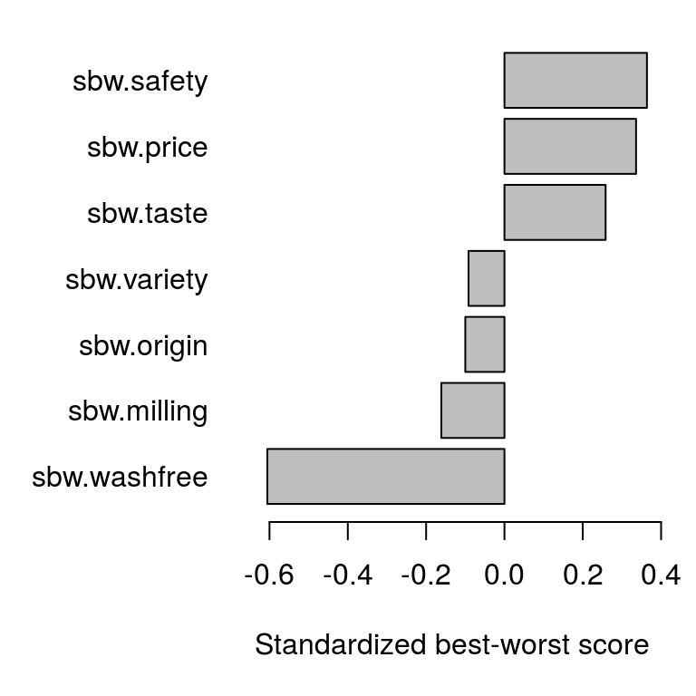
Figure 3.6: Bar plot of mean standardized BW scores
If necessary, three types of error bar are added on the bars using the argument error.bar: the standard deviation ("sd"), the standard error ("se"), and the confidence interval ("ci"). The confidence level is set via the argument conf.level (the default is 0.95) when selecting the confidence interval. If error bars are unnecessary, NULL (the default) is assigned to error.bar.
Other methods, such as sum() and summary() are also available for the S3 class "bws.count2". The sum() method returns the aggregated B, W, BW, and standardized BW scores in data frame format:
##            B   W   BW    stdBW
## origin    67 103  -36 -0.10000
## variety   64  97  -33 -0.09167
## price    160  39  121  0.33611
## taste    125  32   93  0.25833
## safety   153  22  131  0.36389
## washfree  24 242 -218 -0.60556
## milling   37  95  -58 -0.16111
The summary() method calculates (1) aggregated B, W, BW, and standardized BW scores, (2) item ranks based on the BW score, (3) means of B, W, BW, and standardized BW scores, and (4) the square root of the ratio of aggregated B to aggregated W scores and the corresponding standardized scores:
## Number of respondents = 90
##
##            B   W   BW Rank meanB meanW meanBW mean.stdBW sqrtBW std.sqrtBW
## origin    67 103  -36    5 0.744 1.144 -0.400    -0.1000  0.807      0.306
## variety   64  97  -33    4 0.711 1.078 -0.367    -0.0917  0.812      0.308
## price    160  39  121    2 1.778 0.433  1.344     0.3361  2.025      0.768
## taste    125  32   93    3 1.389 0.356  1.033     0.2583  1.976      0.749
## safety   153  22  131    1 1.700 0.244  1.456     0.3639  2.637      1.000
## washfree  24 242 -218    7 0.267 2.689 -2.422    -0.6056  0.315      0.119
## milling   37  95  -58    6 0.411 1.056 -0.644    -0.1611  0.624      0.237
According to the BW scores (BW) or ranking (Rank), the most important characteristic is safety; the second most important is price; and the third most important is taste. The standardized square root of the B/W scores for these three items ranges from 1.00 to 0.75, whereas those for the remaining four items range from 0.31 to 0.12. These results tell us that the rice characteristics of safety, price, and taste are relatively important for the respondents.
3.9.2 The modeling approach
Finally, we fit the conditional logit model to the Case 1 BWS responses on the basis of the maxdiff model. The mlogit() function is used to fit the models. Although this function has many arguments, only two (i.e., formula and data) are used in this example.
When using mlogit() to fit the conditional logit model, the structure of the model formula is similar to that for the linear regression function, lm()—the dependent variable is set on the left-hand side of ~, whereas the independent variables are set on the right-hand side according to a systematic component of the utility function to be fitted. The variable RES corresponds to the dependent variable. Although the item variables correspond to the independent variables, an arbitrary item variable must be omitted from the model because all the item variables are dummy variables. We omit washfree from the model because wash-free rice was found to be the least important item (as shown in the output from the sum() or summary() methods mentioned above). Thus, the systematic component of the utility function for the example under our model settings is
\[\begin{align}
v = \beta_{1}origin + \beta_{2}variety + \beta_{3}price + \beta_{4}taste + \beta_{5}safety + \beta_{6}milling,
\end{align}\]
where \(origin\), \(variety\), \(price\), \(taste\), \(safety\), and \(milling\) are item variables, and \(\beta\)s are coefficients to be estimated. The model formula for mlogit(), corresponding to the systematic component mentioned above, is described (and stored as object mf) as:
Note that the last term “- 1” means that the model has no alternative-specific constants.
The dataset created by the bws.dataset() function has to be converted into that of the S3 class "dfidx" with the dfidx() function in the dfidx package (see the dfidx help document for details on the arguments):
# Data set for the maxdiff model
md.data.dfidx <- dfidx(data = md.data,
                       idx = list(c("STR", "id"), "PAIR"),
                       choice = "RES")
After preparing the dataset for the conditional logit model analysis, we fit the maxdiff model using mlogit() with the model formula mf and the dataset md.data.dfidx:
##
## Call:
## mlogit(formula = RES ~ origin + variety + price + taste + safety +
##     milling - 1, data = md.data.dfidx, method = "nr")
##
## Frequencies of alternatives:choice
##      1      2      3      4      5      6      7      8      9     10     11
## 0.0365 0.0952 0.0825 0.1190 0.1238 0.1222 0.0984 0.0540 0.1476 0.0540 0.0302
##     12
## 0.0365
##
## nr method
## 5 iterations, 0h:0m:0s
## g'(-H)^-1g = 8.32E-06
## successive function values within tolerance limits
##
## Coefficients :
##         Estimate Std. Error z-value Pr(>|z|)
## origin     1.131      0.118    9.60   <2e-16 ***
## variety    1.108      0.116    9.54   <2e-16 ***
## price      2.013      0.126   16.02   <2e-16 ***
## taste      1.847      0.124   14.92   <2e-16 ***
## safety     2.072      0.126   16.42   <2e-16 ***
## milling    0.960      0.115    8.35   <2e-16 ***
## ---
## Signif. codes:  0 '***' 0.001 '**' 0.01 '*' 0.05 '.' 0.1 ' ' 1
##
## Log-Likelihood: -1320
The output from summary(md.out) consists of three blocks: the first block reports the call to the function and frequency of alternatives; the second block reports information regarding the optimization; and the last block reports estimated coefficients and the related statistics, including the value of log-likelihood at convergence. In the third block, column Estimate contains the estimated coefficients; column Std. Error contains the standard error of the estimated coefficients; and columns z-value and Pr(>|z|) respectively give the \(z\) value and \(p\) value under the null hypothesis, in which the coefficient is zero. All variables have significant and positive coefficients. This means that the six characteristics used as the independent variables in the model (i.e., from place of origin to milling date) are more important than the rice being wash-free, which is the base characteristic having a coefficient of zero.
To see the extent of relative importance among the seven characteristics, the share of preferences for them are calculated using bws.sp():
##   origin  variety    price    taste   safety  milling washfree
##  0.09836  0.09609  0.23759  0.20127  0.25203  0.08292  0.03174
This result reveals that safety, which is the most important of the seven characteristics, is approximately 8 times (\(= 0.25203/0.03174\)) as important as rice being wash-free, which is the least important one, and approximately 3 times (\(= 0.25203/0.08292\)) as important as the milling date, which is the second least important characteristic.
Unfortunately, the summary method for the S3 class "mlogit" does not calculate a goodness-of-fit measure for a model such as McFadden’s R-squared (rho-squared) when a model to be fitted has no constant terms. The value of McFadden’s R-squared for our model and its adjusted version are calculated as follows:
LL0 <- - 90 * 7 * log(12) # the value of log-likelihood at zero
LLb <- as.numeric(md.out$logLik) # the value of log-likelihood at convergence
1 - (LLb/LL0)  # McFadden's R-squared
## [1] 0.1581## [1] 0.1543The value of the goodness-of-fit measure for the model does not show a good model fit (see Hensher, Rose, and Greene 2015). This may have occurred because the heterogeneity we saw in the counting approach is not considered in the model.
Therefore, we apply the random parameters logit model to our data (see Appendix 3B for a method including individuals’ characteristics). Assuming that the coefficients of the item variables are normally distributed, Halton sequences are used in the simulation process of the random parameters logit model estimation. The number of draws in the simulation (R below) is 100; and the panel data structure is taken into account in the model (see vignettes of mlogit for details on the arguments). The following code fits the random parameters logit model under our assumptions:
rpl1 <- mlogit(
  formula = RES ~ origin + variety + price + taste + safety + milling - 1| 0,
  data = md.data.dfidx,
  rpar = c(origin = "n", variety = "n", price = "n", taste = "n", safety = "n",
           milling = "n"),
  R = 100, halton = NA, panel = TRUE)
summary(rpl1)
##
## Call:
## mlogit(formula = RES ~ origin + variety + price + taste + safety +
## milling - 1 | 0, data = md.data.dfidx, rpar = c(origin = "n",
## variety = "n", price = "n", taste = "n", safety = "n", milling = "n"),
## R = 100, halton = NA, panel = TRUE)
##
## Frequencies of alternatives:choice
## 1 2 3 4 5 6 7 8 9 10 11
## 0.0365 0.0952 0.0825 0.1190 0.1238 0.1222 0.0984 0.0540 0.1476 0.0540 0.0302
## 12
## 0.0365
##
## bfgs method
## 24 iterations, 0h:0m:11s
## g'(-H)^-1g = 9.32E-07
## gradient close to zero
##
## Coefficients :
## Estimate Std. Error z-value Pr(>|z|)
## origin 1.741 0.155 11.24 <2e-16 ***
## variety 1.787 0.153 11.66 <2e-16 ***
## price 3.989 0.243 16.43 <2e-16 ***
## taste 3.093 0.200 15.48 <2e-16 ***
## safety 3.628 0.198 18.31 <2e-16 ***
## milling 1.638 0.164 10.01 <2e-16 ***
## sd.origin 1.667 0.178 9.35 <2e-16 ***
## sd.variety 1.866 0.179 10.44 <2e-16 ***
## sd.price 2.689 0.238 11.32 <2e-16 ***
## sd.taste 2.007 0.190 10.57 <2e-16 ***
## sd.safety 1.955 0.211 9.26 <2e-16 ***
## sd.milling 1.605 0.187 8.60 <2e-16 ***
## ---
## Signif. codes: 0 '***' 0.001 '**' 0.01 '*' 0.05 '.' 0.1 ' ' 1
##
## Log-Likelihood: -1090
##
## random coefficients
## Min. 1st Qu. Median Mean 3rd Qu. Max.
## origin -Inf 0.6162 1.741 1.741 2.865 Inf
## variety -Inf 0.5286 1.787 1.787 3.046 Inf
## price -Inf 2.1749 3.989 3.989 5.803 Inf
## taste -Inf 1.7387 3.093 3.093 4.447 Inf
## safety -Inf 2.3094 3.628 3.628 4.946 Inf
## milling -Inf 0.5554 1.638 1.638 2.721 InfThe value of McFadden’s R-squared and its adjusted version for the fitted model are given as:
## [1] 0.3018## [1] 0.2941Thus, the goodness-of-fit measures for the random parameters logit model are improved compared with those for the conditional logit model.
The shares of preferences for the seven items calculated using the estimated mean coefficients, from origin to milling, are as follows:
bws.sp(object = rpl1, base = "washfree",
       coef = c("origin", "variety", "price", "taste", "safety", "milling"))
## origin variety price taste safety milling washfree
## 0.043367 0.045423 0.410651 0.167598 0.286218 0.039137 0.007606When fitting the random parameters logit model, the output from mlogit() includes individual-specific parameters in the object indpar:
##   id origin variety price taste safety milling
## 1  1  4.596  1.7906 2.461 2.212  3.691  2.9042
## 2  2  1.573  1.9294 7.589 3.260  4.645  0.9686
## 3  3  1.877  0.7812 4.060 6.235  2.011  1.7814
## 4  4  3.641  1.4637 7.454 3.063  4.472  2.5378
## 5  5  1.635  5.9019 3.040 5.881  3.713  1.9049
## 6  6  2.953  1.5403 7.395 4.639  3.534  2.2141
The function bws.sp() can also calculate the shares of preferences for items by individual on the basis of the individual-specific parameters as follows:
indsp.mlogit <- bws.sp(
  object = rpl1$indpar[, -1], # Variable id is removed
  base = "washfree")
head(indsp.mlogit)
## origin variety price taste safety milling washfree
## [1,] 0.534850 0.032347 0.06324 0.04930 0.21636 0.098505 0.0053974
## [2,] 0.002274 0.003246 0.93143 0.01228 0.04906 0.001242 0.0004714
## [3,] 0.011042 0.003693 0.09805 0.86285 0.01263 0.010040 0.0016907
## [4,] 0.020154 0.002284 0.91278 0.01131 0.04626 0.006688 0.0005286
## [5,] 0.006425 0.457952 0.02617 0.44850 0.05129 0.008413 0.0012522
## [6,] 0.010654 0.002593 0.90459 0.05748 0.01904 0.005087 0.0005558Appendix 3A: Creating alternative datasets for analysis
The code chunks for creating datasets for the marginal and marginal sequential models are as follows:
# Dataset for the marginal model
mr.data <- bws.dataset(
   data = ricebws1,
   response.type = 1,
   choice.sets = des,
   design.type = 2,
   item.names = items.rice,
   id = "id",
   response = response.vars,
   model = "marginal") # the marginal model
# Dataset for the marginal sequential model
sq.data <- bws.dataset(
   data = ricebws1,
   response.type = 1,
   choice.sets = des,
   design.type = 2,
   item.names = items.rice,
   id = "id",
   response = response.vars,
   model = "sequential") # the marginal sequential model
The data frame mr.data consists of 5,040 rows (= 90 respondents \(\times\) 7 BWS questions \(\times\) 8 possible best and worst items per BWS question [= 4 possible best items \(+\) 4 possible worst items]) and 19 columns (variables):
## [1] 5040 19The following output displays the 19 variables in mr.data corresponding to the 8 possible best and worst items in the first question (Q = 1) for respondent 1 (id = 1). The first four rows show the possible best item (BW = 1), whereas the last four rows show the possible worst items (BW = -1). The column Item shows the possible best and worst items in item number format—e.g., the first row in the following output indicates that variety (item number = 2) is treated as the possible best characteristic, whereas the last row indicates that milling (item number = 7) is treated as the possible worst characteristic. The item variables are created as dummy variables with reversed sign when the items are treated as the possible worst. Therefore, the first row indicates that the value of the item variable variety is 1 and the values of the remaining item variables are 0, whereas the last row indicates that the value of the item variable milling is -1 and the values of the remaining item variables are 0. According to the values of column RES, respondent 1 selected milling date and variety as the best and worst characteristics in the first question.
##   id Q ALT BW Item RES.B RES.W   RES origin variety price taste safety washfree
## 1  1 1   1  1    2     7     2 FALSE      0       1     0     0      0        0
## 2  1 1   2  1    3     7     2 FALSE      0       0     1     0      0        0
## 3  1 1   3  1    4     7     2 FALSE      0       0     0     1      0        0
## 4  1 1   4  1    7     7     2  TRUE      0       0     0     0      0        0
## 5  1 1   1 -1    2     7     2  TRUE      0      -1     0     0      0        0
## 6  1 1   2 -1    3     7     2 FALSE      0       0    -1     0      0        0
## 7  1 1   3 -1    4     7     2 FALSE      0       0     0    -1      0        0
## 8  1 1   4 -1    7     7     2 FALSE      0       0     0     0      0        0
##   milling  STR age hp chem
## 1       0 1011   3  2    1
## 2       0 1011   3  2    1
## 3       0 1011   3  2    1
## 4       1 1011   3  2    1
## 5       0 1012   3  2    1
## 6       0 1012   3  2    1
## 7       0 1012   3  2    1
## 8      -1 1012   3  2    1
The data frame sq.data consists of 4,410 rows (= 90 respondents \(\times\) 7 BWS questions \(\times\) 7 possible best and worst items per BWS question [\(= 4\) possible best items \(+\ 3\) possible worst items]) and 19 columns (variables):
## [1] 4410 19The following output shows the 19 variables in sq.data corresponding to the 7 possible best and worst items in the first question (Q = 1) for respondent 1 (id = 1). The row structure in sq.data differs slightly from that in mr.data; specifically, the first four rows correspond to the four possible best items (BW = 1), whereas the last three rows correspond to the three possible worst items (BW = -1)—i.e., the row corresponding to the item selected as the best by the respondent is omitted from the rows corresponding to the possible worst items. In this case, respondent 1 selected milling date as the best characteristic, so the row corresponding to milling is omitted from the rows corresponding to the possible worst item. The definition of item variables is the same as that in the mr.data.
##   id Q ALT BW Item RES.B RES.W   RES origin variety price taste safety washfree
## 1  1 1   1  1    2     7     2 FALSE      0       1     0     0      0        0
## 2  1 1   2  1    3     7     2 FALSE      0       0     1     0      0        0
## 3  1 1   3  1    4     7     2 FALSE      0       0     0     1      0        0
## 4  1 1   4  1    7     7     2  TRUE      0       0     0     0      0        0
## 5  1 1   1 -1    2     7     2  TRUE      0      -1     0     0      0        0
## 6  1 1   2 -1    3     7     2 FALSE      0       0    -1     0      0        0
## 7  1 1   3 -1    4     7     2 FALSE      0       0     0    -1      0        0
##   milling  STR age hp chem
## 1       0 1011   3  2    1
## 2       0 1011   3  2    1
## 3       0 1011   3  2    1
## 4       1 1011   3  2    1
## 5       0 1012   3  2    1
## 6       0 1012   3  2    1
## 7       0 1012   3  2    1
The datasets mr.data and sq.data are respectively converted into that of the S3 class "dfidx" as follows:
# Dataset for the marginal model
mr.data.dfidx <- dfidx(data = mr.data,
                       idx = list(c("STR", "id"), "ALT"),
                       choice = "RES")
# Dataset for the marginal sequential model
sq.data.dfidx <- dfidx(data = sq.data,
                       idx = list(c("STR", "id"), "ALT"),
                       choice = "RES")
The marginal model is fit using mlogit() with the following code:
##
## Call:
## mlogit(formula = RES ~ origin + variety + price + taste + safety +
##     milling - 1, data = mr.data.dfidx, method = "nr")
##
## Frequencies of alternatives:choice
##     1     2     3     4
## 0.243 0.243 0.278 0.237
##
## nr method
## 4 iterations, 0h:0m:0s
## g'(-H)^-1g = 3.31E-07
## gradient close to zero
##
## Coefficients :
##         Estimate Std. Error z-value Pr(>|z|)
## origin     1.377      0.128   10.73   <2e-16 ***
## variety    1.339      0.127   10.56   <2e-16 ***
## price      2.493      0.133   18.69   <2e-16 ***
## taste      2.286      0.132   17.29   <2e-16 ***
## safety     2.568      0.134   19.17   <2e-16 ***
## milling    1.149      0.125    9.18   <2e-16 ***
## ---
## Signif. codes:  0 '***' 0.001 '**' 0.01 '*' 0.05 '.' 0.1 ' ' 1
##
## Log-Likelihood: -1430
The marginal sequential model is fit using mlogit() with the following code:
##
## Call:
## mlogit(formula = RES ~ origin + variety + price + taste + safety +
##     milling - 1, data = sq.data.dfidx, method = "nr")
##
## Frequencies of alternatives:choice
##     1     2     3     4
## 0.243 0.243 0.278 0.237
##
## nr method
## 5 iterations, 0h:0m:0s
## g'(-H)^-1g = 1.99E-06
## successive function values within tolerance limits
##
## Coefficients :
##         Estimate Std. Error z-value Pr(>|z|)
## origin     1.313      0.134    9.80   <2e-16 ***
## variety    1.276      0.132    9.66   <2e-16 ***
## price      2.338      0.140   16.65   <2e-16 ***
## taste      2.172      0.138   15.70   <2e-16 ***
## safety     2.432      0.141   17.30   <2e-16 ***
## milling    1.150      0.129    8.92   <2e-16 ***
## ---
## Signif. codes:  0 '***' 0.001 '**' 0.01 '*' 0.05 '.' 0.1 ' ' 1
##
## Log-Likelihood: -1310
The resultant shares of preferences for the seven characteristics are similar among the three models:
sp.mr <- bws.sp(object = mr.out, base = "washfree")
sp.sq <- bws.sp(object = sq.out, base = "washfree")
(sp.all <- cbind(sp.md, sp.mr, sp.sq))
## sp.md sp.mr sp.sq
## origin 0.09836 0.08454 0.08854
## variety 0.09609 0.08133 0.08535
## price 0.23759 0.25788 0.24690
## taste 0.20127 0.20971 0.20902
## safety 0.25203 0.27795 0.27112
## milling 0.08292 0.06727 0.07525
## washfree 0.03174 0.02132 0.02382## sp.md sp.mr sp.sq
## sp.md 1.0000 0.9982 0.9990
## sp.mr 0.9982 1.0000 0.9994
## sp.sq 0.9990 0.9994 1.0000Appendix 3B: Incorporating individuals’ characteristics
A random parameters logit model with considering the effect of respondents’ attitudes toward low-agrochemicals on the mean parameters is fitted using the gmnl() function in the gmnl package (Sarrias and Daziano 2017):
Although the current version of mlogit package deprecates the mlogit.data() function (see the mlogit help document), the gmnl() function needs a dataset of the S3 class "mlogit.data". Therefore, after converting the dataset md.data into that of S3 class "mlogit.data", the random parameter logit model is fitted:
md.data.ml <- mlogit.data(data = md.data, choice = "RES", shape = "long",
                          alt.var = "PAIR", chid.var = "STR", id.var = "id")
rpl2 <- gmnl(RES ~ origin + variety + price + taste + safety + milling|0|0|chem - 1,
             data = md.data.ml,
             ranp = c(origin = "n", variety = "n", price = "n", taste = "n",
                      safety = "n", milling = "n"),
             mvar = list(origin = "chem", variety = "chem", price = "chem",
                         taste = "chem", safety = "chem", milling = "chem"),
             model = "mixl",
             R = 100, halton = NA, panel = TRUE)
## Estimating MIXL model##
## Model estimated on: 月 3月 29 15時01分47秒 2021
##
## Call:
## gmnl(formula = RES ~ origin + variety + price + taste + safety +
## milling | 0 | 0 | chem - 1, data = md.data.ml, model = "mixl",
## ranp = c(origin = "n", variety = "n", price = "n", taste = "n",
## safety = "n", milling = "n"), R = 100, haltons = NA,
## mvar = list(origin = "chem", variety = "chem", price = "chem",
## taste = "chem", safety = "chem", milling = "chem"), panel = TRUE,
## method = "bfgs")
##
## Frequencies of categories:
##
## 1 2 3 4 5 6 7 8 9 10 11
## 0.0365 0.0952 0.0825 0.1190 0.1238 0.1222 0.0984 0.0540 0.1476 0.0540 0.0302
## 12
## 0.0365
##
## The estimation took: 0h:1m:3s
##
## Coefficients:
## Estimate Std. Error z-value Pr(>|z|)
## origin 1.356 0.343 3.96 7.6e-05 ***
## variety 1.510 0.329 4.59 4.5e-06 ***
## price 3.789 0.462 8.19 2.2e-16 ***
## taste 2.240 0.373 6.01 1.9e-09 ***
## safety 2.221 0.324 6.86 6.8e-12 ***
## milling 1.217 0.292 4.16 3.2e-05 ***
## origin.chem 0.524 0.427 1.23 0.21989
## variety.chem 0.393 0.458 0.86 0.39060
## price.chem 0.567 0.564 1.00 0.31496
## taste.chem 1.611 0.477 3.38 0.00073 ***
## safety.chem 1.549 0.441 3.51 0.00045 ***
## milling.chem 0.408 0.374 1.09 0.27514
## sd.origin 1.579 0.196 8.06 8.9e-16 ***
## sd.variety 1.408 0.166 8.51 < 2e-16 ***
## sd.price 2.927 0.328 8.91 < 2e-16 ***
## sd.taste 1.890 0.223 8.47 < 2e-16 ***
## sd.safety 1.665 0.234 7.12 1.0e-12 ***
## sd.milling 1.165 0.156 7.46 8.5e-14 ***
## ---
## Signif. codes: 0 '***' 0.001 '**' 0.01 '*' 0.05 '.' 0.1 ' ' 1
##
## Optimization of log-likelihood by BFGS maximization
## Log Likelihood: -1100
## Number of observations: 630
## Number of iterations: 67
## Exit of MLE: successful convergence
## Simulation based on 100 drawsAs shown above, respondents’ attitudes toward low-agrochemicals have significant effects on the mean parameters regarding taste and safety.
The shares of preferences for the seven characteristics based on the estimated mean coefficients, from origin to milling, are calculated as follows:
bws.sp(object = rpl2, base = "washfree",
       coef = c("origin", "variety", "price", "taste", "safety", "milling"))
## origin variety price taste safety milling washfree
## 0.05134 0.05989 0.58472 0.12423 0.12192 0.04466 0.01323The individual-specific parameters for the random parameters logit model are calculated by applying the function effect.gmnl() to the output from gmnl() (see Sarrias and Daziano (2017) for details on effect.gmnl()):
##      origin variety price taste safety milling
## [1,]  3.123   1.483 1.760 2.759  4.365   2.995
## [2,]  1.762   2.448 7.446 4.196  4.437   1.305
## [3,]  2.586   1.955 5.000 6.696  3.628   1.288
## [4,]  1.903   1.119 6.229 1.374  3.934   1.479
## [5,]  2.357   3.934 3.845 4.684  3.156   2.608
## [6,]  2.606   1.699 6.846 4.892  3.335   1.331
Accordingly, the shares of preferences for items by individual are calculated using bws.sp() as follows:
##        origin  variety   price    taste  safety  milling  washfree
## [1,] 0.153125 0.029712 0.03919 0.106350 0.53017 0.134712 0.0067404
## [2,] 0.003089 0.006130 0.90826 0.035207 0.04483 0.001955 0.0005302
## [3,] 0.013017 0.006927 0.14549 0.793166 0.03687 0.003552 0.0009801
## [4,] 0.011621 0.005301 0.87840 0.006843 0.08849 0.007605 0.0017322
## [5,] 0.041439 0.200698 0.18355 0.424949 0.09216 0.053278 0.0039256
## [6,] 0.012038 0.004860 0.83553 0.118372 0.02495 0.003362 0.0008883
References
Aizaki, H. 2021. Support.BWS: Tools for Case 1 Best-Worst Scaling. https://CRAN.R-project.org/package=support.BWS.
Cochran, W. G., and G. M. Cox. 1957. Experimental Designs. 2nd ed. New Jersey, USA: John Wiley & Sons.
Cohen, E. 2009. “Applying Best-Worst Scaling to Wine Marketing.” International Journal of Wine Business Research 21 (1): 8–23. https://doi.org/10.1108/17511060910948008.
Cohen, S. H. 2003. “Maximum Difference Scaling: Improved Measures of Importance and Preference for Segmentation.” Sawtooth Software Research Research Paper Series, 1–17. https://sawtoothsoftware.com/resources/technical-papers/maximum-difference-scaling-improved-measures-of-importance-and-preference-for--segmentation.
Cohen, S., and L. Neira. 2004. “Measuring Preferences for Product Benefits Across Countries: Overcoming Scale Usage Bias with Maximum Difference Scaling.” Excellence in International Research, 1–22.
Croissant, Y. 2020a. Dfidx: Indexed Data Frames. https://CRAN.R-project.org/package=dfidx.
Croissant, Y. 2020b. “Estimation of Random Utility Models in R: The Mlogit Package.” Journal of Statistical Software 95 (11): 1–41. https://doi.org/10.18637/jss.v095.i11.
Dumbrell, N. P., M. E. Kragt, and F. L. Gibson. 2016. “What Carbon Farming Activities Are Farmers Likely to Adopt? A Best–Worst Scaling Survey.” Land Use Policy 54: 29–37. https://doi.org/10.1016/j.landusepol.2016.02.002.
Finn, A., and J. J. Louviere. 1992. “Determining the Appropriate Response to Evidence of Public Concern: The Case of Food Safety.” Journal of Public Policy & Marketing, 12–25. https://doi.org/10.1177/074391569201100202.
Flynn, T. N., J. J. Louviere, T. J. Peters, and J. Coast. 2007. “Best–Worst Scaling: What It Can Do for Health Care Research and How to Do It.” Journal of Health Economics 26 (1): 171–89. https://doi.org/10.1016/j.jhealeco.2006.04.002.
Flynn, T. 2008. “Estimating Preferences for a Dermatology Consultation Using Best–Worst Scaling: Comparison of Various Methods of Analysis.” BMC Medical Research Methodology 8 (1): 76. https://doi.org/10.1186/1471-2288-8-76.
Gallego, G., J. F. P. Bridges, T. Flynn, B. M. Blauvelt, and L. W. Niessen. 2012. “Using Best-Worst Scaling in Horizon Scanning for Hepatocellular Carcinoma Technologies.” International Journal of Technology Assessment in Health Care 28 (3): 339–46. https://doi.org/10.1017/S026646231200027X.
Hein, K. A., S. R. Jaeger, B. T. Carr, and C. M. Delahunty. 2008. “Comparison of Five Common Acceptance and Preference Methods.” Food Quality and Preference 19 (7): 651–61. https://doi.org/10.1016/j.foodqual.2008.06.001.
Hensher, D. A., J. M. Rose, and W. H. Greene. 2015. Applied Choice Analysis. 2nd ed. Cambridge, UK: Cambridge University Press.
Hoek, J., P. Gendall, L. Rapson, and J. Louviere. 2011. “Information Accessibility and Consumers’ Knowledge of Prescription Drug Benefits and Risks.” Journal of Consumer Affairs 45 (2): 248–74. https://doi.org/10.1111/j.1745-6606.2011.01202.x.
Jaeger, S. R., and A. V. Cardello. 2009. “Direct and Indirect Hedonic Scaling Methods: A Comparison of the Labeled Affective Magnitude (Lam) Scale and Best–Worst Scaling.” Food Quality and Preference 20 (3): 249–58. https://doi.org/10.1016/j.foodqual.2008.10.005.
Jaeger, S. R., P. J. Danaher, and R. J. Brodie. 2009. “Wine Purchase Decisions and Consumption Behaviours: Insights from a Probability Sample Drawn in Auckland, New Zealand.” Food Quality and Preference 20 (4): 312–19. https://doi.org/https://doi.org/10.1016/j.foodqual.2009.02.003.
Lee, J. A., G. N. Soutar, and J. Louviere. 2007a. “Measuring Values Using Best-Worst Scaling: The Lov Example.” Psychology & Marketing 24 (12): 1043–58. https://doi.org/10.1002/mar.20197.
Lee, J. 2007b. “Measuring Values Using Best-Worst Scaling: The Lov Example.” Psychology & Marketing 24 (12): 1043–58. https://doi.org/10.1002/mar.20197.
Loureiro, M. L., and F. D. Arcos. 2012. “Applying Best–Worst Scaling in a Stated Preference Analysis of Forest Management Programs.” Journal of Forest Economics 18 (4): 381–94. https://doi.org/10.1016/j.jfe.2012.06.006.
Louviere, J. J., T. N. Flynn, and A. A. J. Marley. 2015. Best–Worst Scaling: Theory, Methods and Applications. Cambridge, UK: Cambridge University Press.
Lusk, J. L., and B. C. Briggeman. 2009. “Food Values.” American Journal of Agricultural Economics 91: 184–96. https://doi.org/10.1111/j.1467-8276.2008.01175.x.
Mazanov, J., T. Huybers, and J. Connor. 2012. “Prioritising Health in Anti-Doping: What Australians Think.” Journal of Science and Medicine in Sport 15 (5): 381–85. https://doi.org/10.1016/j.jsams.2012.02.007.
Mueller, S., I. L. Francis, and L. Lockshin. 2009. “Comparison of Best–Worst and Hedonic Scaling for the Measurement of Consumer Wine Preferences.” Australian Journal of Grape and Wine Research 15 (3): 205–15. https://doi.org/10.1111/j.1755-0238.2009.00049.x.
R Core Team. 2021a. An Introduction to R. https://CRAN.R-project.org/manuals.html.
R Core Team. 2021b. R: A Language and Environment for Statistical Computing. Vienna, Austria: R Foundation for Statistical Computing. https://www.R-project.org/.
Sailer, M. O. 2013. Crossdes: Construction of Crossover Designs. https://CRAN.R-project.org/package=crossdes.
Sarrias, M., and R. Daziano. 2017. “Multinomial Logit Models with Continuous and Discrete Individual Heterogeneity in R: The Gmnl Package.” Journal of Statistical Software, Articles 79 (2): 1–46. https://doi.org/10.18637/jss.v079.i02.
Wang, T., B. Wong, A. Huang, P. Khatri, C. Ng, M. Forgie, J. H. Lanphear, and P. J. O’Neill. 2011. “Factors Affecting Residency Rank-Listing: A Maxdiff Survey of Graduating Canadian Medical Students.” BMC Medical Education 11 (1): 61. https://doi.org/10.1186/1472-6920-11-61.